HMM Based Trading Applications
HMM Based Trading Applications
From Regime Detection to Profitable Trading Strategies
See the Notebook source on GitHub.
Your Journey So Far
Notebook 1: Why Use Log Returns?
You learned WHY log returns are necessary:
- Stationarity, additivity, scale invariance
- Mathematical properties required for HMMs
Notebook 2: HMM Basics
You learned HOW HMMs work:
- Hidden states, transition matrices, emissions
- Viterbi and forward-backward algorithms
Notebook 3: Hidden Regime Pipeline
You learned to DETECT regimes:
- Pipeline setup and execution
- Regime classification and duration
- Model selection and validation
Notebook 4: Trading Applications (This Notebook)
You’ll learn to TRADE using regimes:
- Risk management by regime
- Technical indicator integration
- Position sizing and signal generation
- Backtesting and validation
What This Notebook Covers
Part A: Regime-Specific Risk Analysis (Sections 1-2) Part B: Technical Indicator Integration (Sections 3-4) Part C: Portfolio Applications (Sections 5-6) Part D: Backtesting & Validation (Sections 7-8) Part E: Best Practices & Conclusion (Section 9)
Prerequisites
Before starting this notebook:
- ✓ Completed Notebook 03
- ✓ Understand regime detection pipeline
- ✓ Familiar with confidence levels and regime characteristics
Important: This notebook demonstrates trading concepts for educational purposes. Always backtest thoroughly and start with paper trading before risking real capital.
 1import sys
 2from pathlib import Path
 3import numpy as np
 4import pandas as pd
 5import matplotlib.pyplot as plt
 6import seaborn as sns
 7from datetime import datetime, timedelta
 8import warnings
 9warnings.filterwarnings('ignore')
10
11# Add parent to path
12sys.path.insert(0, str(Path().absolute().parent))
13
14# Import hidden_regime
15import hidden_regime as hr
16
17# Plotting
18plt.style.use('seaborn-v0_8-whitegrid')
19sns.set_palette(sns.color_palette())
20
21print(f"Imports complete")
22print(f"hidden-regime version: {hr.__version__}")
Imports complete
hidden-regime version: 1.0.0
Setup: Run Pipeline from Notebook 03
We’ll reuse the same NVDA example to demonstrate trading applications.
 1# Create pipeline (same as Notebook 03)
 2ticker = 'NVDA'
 3n_states = 3
 4
 5pipeline = hr.create_financial_pipeline(
 6    ticker=ticker,
 7    n_states=n_states,
 8    include_report=False
 9)
10
11# Execute pipeline
12report = pipeline.update()
13result = pipeline.component_outputs['analysis']
14raw_data = pipeline.data.get_all_data()
15
16print(f"Pipeline complete: {len(result)} days analyzed")
17print(f"Date range: {result.index[0].date()} to {result.index[-1].date()}")
Training on 500 observations (removed 0 NaN values)
Pipeline complete: 500 days analyzed
Date range: 2023-10-18 to 2025-10-15
Part A: Regime-Specific Risk Analysis
1. Risk Metrics by Regime
Different regimes have different risk characteristics. Understanding these helps with:
- Position sizing: Larger positions in low-risk regimes
- Stop-loss placement: Wider stops in high-volatility regimes
- Strategy selection: Trend-following vs mean-reversion
Key Risk Metrics
Value at Risk (VaR): Maximum expected loss at confidence level $\alpha$
$ \text{VaR}_\alpha = -F^{-1}(\alpha) $
where $F^{-1}$ is the inverse CDF of returns.
Expected Shortfall (ES): Average loss beyond VaR
$ \text{ES}_\alpha = E[r \mid r \leq -\text{VaR}_\alpha] $
Sharpe Ratio: Risk-adjusted return
$ \text{Sharpe} = \frac{\mu - r_f}{\sigma} $
where $\mu$ is mean return, $r_f$ is risk-free rate, $\sigma$ is volatility.
Maximum Drawdown: Largest peak-to-trough decline
$ \text{MDD} = \max_{t} \left[ \frac{\max_{\tau \leq t} P_\tau - P_t}{\max_{\tau \leq t} P_\tau} \right] $
 1# Get log returns aligned with regimes
 2log_return_col = next((col for col in raw_data.columns if col.lower() == 'log_return'), None)
 3
 4if log_return_col is None:
 5    raise ValueError("Could not find log_return column")
 6
 7# Calculate comprehensive risk metrics by regime
 8risk_metrics = {}
 9
10for regime in sorted(result['regime_name'].unique()):
11    regime_data = result[result['regime_name'] == regime]
12    regime_indices = regime_data.index
13    regime_returns = raw_data.loc[regime_indices, log_return_col].dropna()
14
15    if len(regime_returns) < 2:
16        continue
17
18    # Basic statistics
19    mean_daily = regime_returns.mean()
20    std_daily = regime_returns.std()
21    mean_annual = mean_daily * 252
22    std_annual = std_daily * np.sqrt(252)
23
24    # Sharpe ratio (assuming 0% risk-free rate)
25    sharpe = (mean_annual / std_annual) if std_annual > 0 else 0
26
27    # Maximum drawdown
28    cumulative = (1 + regime_returns).cumprod()
29    running_max = cumulative.expanding().max()
30    drawdown = (cumulative - running_max) / running_max
31    max_drawdown = drawdown.min()
32
33    # Value at Risk
34    var_95 = np.percentile(regime_returns, 5)
35    var_99 = np.percentile(regime_returns, 1)
36
37    # Expected Shortfall (Conditional VaR)
38    es_95 = regime_returns[regime_returns <= var_95].mean()
39    es_99 = regime_returns[regime_returns <= var_99].mean()
40
41    # Win rate and profit factor
42    wins = regime_returns[regime_returns > 0]
43    losses = regime_returns[regime_returns < 0]
44    win_rate = len(wins) / len(regime_returns) if len(regime_returns) > 0 else 0
45    total_wins = wins.sum() if len(wins) > 0 else 0
46    total_losses = abs(losses.sum()) if len(losses) > 0 else 0
47    profit_factor = total_wins / total_losses if total_losses > 0 else float('inf')
48
49    risk_metrics[regime] = {
50        'days': len(regime_returns),
51        'mean_daily': mean_daily * 100,
52        'std_daily': std_daily * 100,
53        'mean_annual': mean_annual * 100,
54        'std_annual': std_annual * 100,
55        'sharpe': sharpe,
56        'max_drawdown': max_drawdown * 100,
57        'var_95': var_95 * 100,
58        'var_99': var_99 * 100,
59        'es_95': es_95 * 100,
60        'es_99': es_99 * 100,
61        'win_rate': win_rate * 100,
62        'profit_factor': profit_factor
63    }
64
65# Display risk metrics table
66print("Risk Metrics by Regime")
67print("=" * 100)
68print(f"{'Regime':<12} {'Days':<8} {'Ann Return':<12} {'Ann Vol':<12} {'Sharpe':<10} {'Max DD':<12}")
69print("-" * 100)
70
71for regime in sorted(risk_metrics.keys()):
72    m = risk_metrics[regime]
73    print(f"{regime:<12} {m['days']:<8} {m['mean_annual']:>10.1f}% {m['std_annual']:>10.1f}% "
74          f"{m['sharpe']:>9.2f} {m['max_drawdown']:>10.1f}%")
75
76print("=" * 100)
Risk Metrics by Regime
====================================================================================================
Regime       Days     Ann Return   Ann Vol      Sharpe     Max DD
----------------------------------------------------------------------------------------------------
Bear         97           -258.0%       68.4%     -3.77      -71.5%
Bull         110           657.7%       20.0%     32.91       -0.0%
Sideways     293           -39.1%       21.9%     -1.78      -44.1%
====================================================================================================
 1# Visualize risk metrics
 2fig, axes = plt.subplots(2, 2, figsize=(16, 10))
 3
 4# Get regime colors
 5from hidden_regime.visualization import get_regime_colors
 6unique_regimes = sorted(risk_metrics.keys())
 7color_list = get_regime_colors(len(unique_regimes), color_scheme="colorblind_safe")
 8regime_colors = dict(zip(unique_regimes, color_list))
 9
10# 1. Sharpe Ratio comparison
11ax = axes[0, 0]
12regimes = list(risk_metrics.keys())
13sharpes = [risk_metrics[r]['sharpe'] for r in regimes]
14colors = [regime_colors[r] for r in regimes]
15
16bars = ax.bar(regimes, sharpes, color=colors, alpha=0.7, edgecolor='black', linewidth=1.5)
17ax.axhline(y=0, color='black', linestyle='-', linewidth=0.8)
18ax.axhline(y=1, color='green', linestyle='--', alpha=0.5, label='Sharpe > 1')
19ax.set_ylabel('Sharpe Ratio', fontsize=12)
20ax.set_title('Risk-Adjusted Returns by Regime', fontsize=14, fontweight='bold')
21ax.grid(True, alpha=0.3, axis='y')
22ax.legend()
23
24# Add value labels
25for bar, val in zip(bars, sharpes):
26    height = bar.get_height()
27    ax.text(bar.get_x() + bar.get_width()/2, height + 0.05,
28            f'{val:.2f}', ha='center', va='bottom', fontweight='bold')
29
30# 2. Volatility comparison
31ax = axes[0, 1]
32vols = [risk_metrics[r]['std_annual'] for r in regimes]
33bars = ax.bar(regimes, vols, color=colors, alpha=0.7, edgecolor='black', linewidth=1.5)
34ax.set_ylabel('Annualized Volatility (%)', fontsize=12)
35ax.set_title('Volatility by Regime', fontsize=14, fontweight='bold')
36ax.grid(True, alpha=0.3, axis='y')
37
38for bar, val in zip(bars, vols):
39    height = bar.get_height()
40    ax.text(bar.get_x() + bar.get_width()/2, height + 1,
41            f'{val:.1f}%', ha='center', va='bottom', fontweight='bold')
42
43# 3. VaR and ES comparison
44ax = axes[1, 0]
45x = np.arange(len(regimes))
46width = 0.35
47
48var_95_vals = [risk_metrics[r]['var_95'] for r in regimes]
49es_95_vals = [risk_metrics[r]['es_95'] for r in regimes]
50
51ax.bar(x - width/2, var_95_vals, width, label='VaR 95%', alpha=0.7, edgecolor='black')
52ax.bar(x + width/2, es_95_vals, width, label='ES 95%', alpha=0.7, edgecolor='black')
53
54ax.set_ylabel('Loss (%)', fontsize=12)
55ax.set_title('Tail Risk Metrics (95% Confidence)', fontsize=14, fontweight='bold')
56ax.set_xticks(x)
57ax.set_xticklabels(regimes)
58ax.legend()
59ax.grid(True, alpha=0.3, axis='y')
60ax.axhline(y=0, color='black', linestyle='-', linewidth=0.8)
61
62# 4. Win rate and profit factor
63ax = axes[1, 1]
64win_rates = [risk_metrics[r]['win_rate'] for r in regimes]
65
66bars = ax.bar(regimes, win_rates, color=colors, alpha=0.7, edgecolor='black', linewidth=1.5)
67ax.axhline(y=50, color='gray', linestyle='--', alpha=0.5, label='50% baseline')
68ax.set_ylabel('Win Rate (%)', fontsize=12)
69ax.set_title('Win Rate by Regime', fontsize=14, fontweight='bold')
70ax.grid(True, alpha=0.3, axis='y')
71ax.legend()
72ax.set_ylim(0, 100)
73
74for bar, val in zip(bars, win_rates):
75    height = bar.get_height()
76    ax.text(bar.get_x() + bar.get_width()/2, height + 2,
77            f'{val:.1f}%', ha='center', va='bottom', fontweight='bold')
78
79plt.tight_layout()
80plt.show()
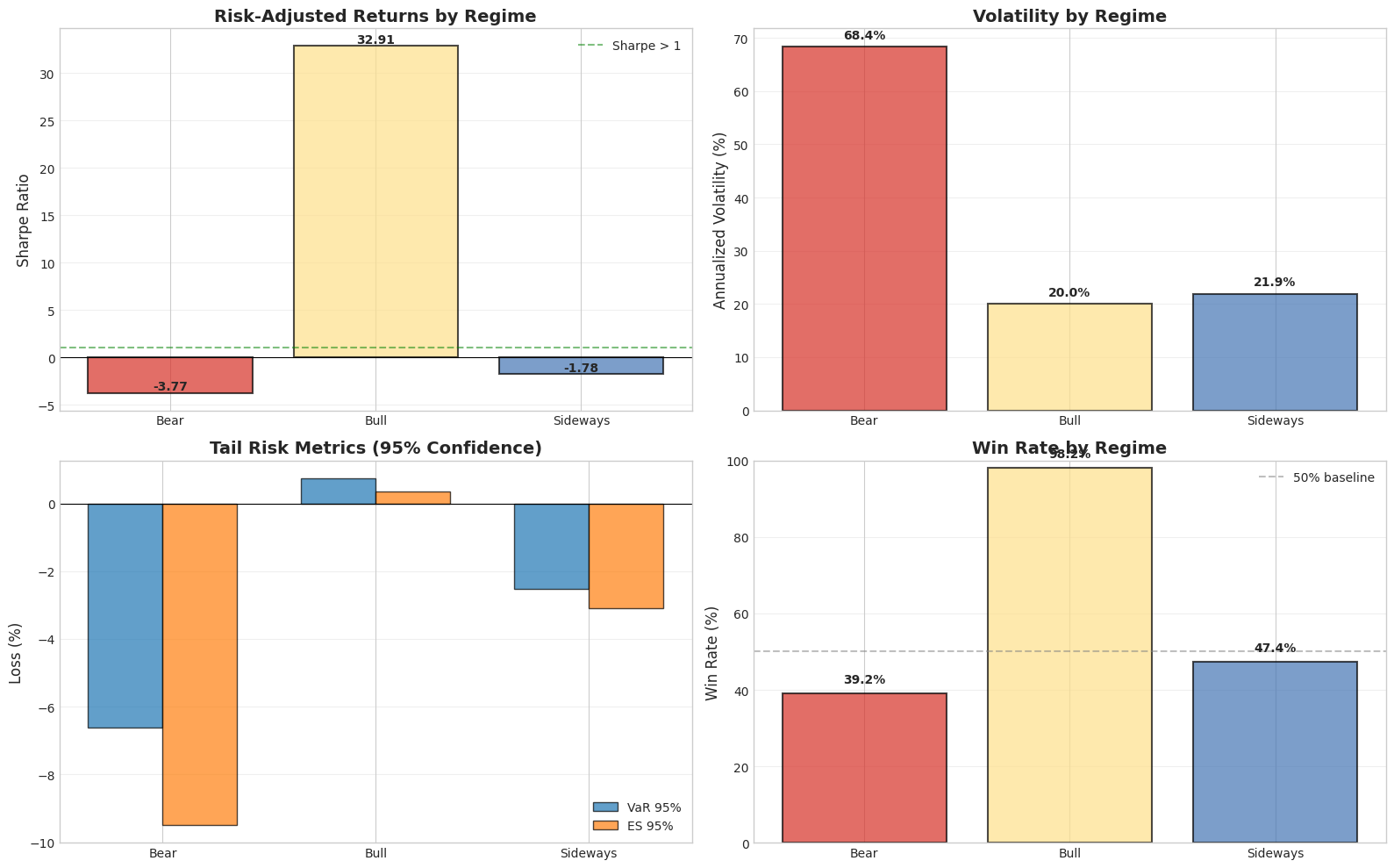
Interpretation & Trading Implications
Sharpe Ratio Analysis:
- Best regime: Highest Sharpe ratio → allocate more capital
- Sharpe > 1: Excellent risk-adjusted returns
- Sharpe < 0: Losing money on average → avoid or short
Volatility Management:
- High volatility regimes: Use wider stop-losses, smaller positions
- Low volatility regimes: Can use tighter stops, larger positions
- Position size ∝ $\frac{1}{\sigma}$ (inverse volatility scaling)
Tail Risk (VaR/ES):
- Expected Shortfall > VaR: Fat-tailed distribution, expect worse losses
- Use ES for position sizing: $\text{Position Size} = \frac{\text{Risk Budget}}{|ES|}$
Win Rate:
- High win rate: Many small wins (mean-reversion strategy)
- Low win rate: Few large wins (trend-following strategy)
- Combine with profit factor for complete picture"
2. Dynamic Position Sizing
Regime-Based Position Sizing Formula
Combine multiple risk factors to determine optimal position size:
$ \text{Position} = \text{Base} \times \underbrace{\frac{\sigma_{\text{target}}}{\sigma_{\text{regime}}}}_{\text{Vol Scaling}} \times \underbrace{\text{Confidence}}_{\text{Regime Certainty}} \times \underbrace{f(\text{Sharpe})}_{\text{Risk-Adjusted}} $
Where:
- Base: Standard position size (e.g., 100% for full allocation)
- Vol Scaling: Adjust for regime volatility
- Confidence: Current regime probability from HMM
- Risk-Adjusted: Additional scaling based on Sharpe ratio
Implementation Strategy
- Set target volatility: $\sigma_{\text{target}} = 15\%$ (annual)
- Scale by regime volatility: Position $\propto \frac{1}{\sigma_{\text{regime}}}$
- Apply confidence filter: Reduce positions when confidence < 70%
- Apply regime quality filter: Reduce positions in negative Sharpe regimes
 1# Calculate position sizing for each day
 2target_vol = 15.0  # Target 15% annualized volatility
 3position_sizes = []
 4
 5for idx in result.index:
 6    current_regime = result.loc[idx, 'regime_name']
 7    confidence = result.loc[idx, 'confidence']
 8
 9    # Get regime metrics
10    regime_vol = risk_metrics[current_regime]['std_annual']
11    regime_sharpe = risk_metrics[current_regime]['sharpe']
12
13    # Base position (100% = full allocation)
14    base_position = 1.0
15
16    # Volatility scaling
17    vol_scalar = target_vol / regime_vol if regime_vol > 0 else 0
18    vol_scalar = min(vol_scalar, 2.0)  # Cap at 2x leverage
19
20    # Confidence scaling
21    conf_scalar = confidence if confidence > 0.6 else confidence * 0.5  # Penalize low confidence
22
23    # Sharpe-based scaling
24    if regime_sharpe > 1.0:
25        sharpe_scalar = 1.0  # Full position
26    elif regime_sharpe > 0.5:
27        sharpe_scalar = 0.75  # Reduce position
28    elif regime_sharpe > 0:
29        sharpe_scalar = 0.5  # Half position
30    else:
31        sharpe_scalar = 0.0  # No position in negative Sharpe regimes
32
33    # Combined position size
34    final_position = base_position * vol_scalar * conf_scalar * sharpe_scalar
35    final_position = max(0, min(final_position, 2.0))  # Clamp to [0, 2]
36
37    position_sizes.append(final_position)
38
39# Add to results (AFTER loop completes)
40result['calculated_position_size'] = position_sizes
41
42# Display summary
43print("Position Sizing Summary")
44print("=" * 80)
45print(f"Target Volatility: {target_vol}%")
46print(f"\nPosition Size Statistics:")
47print(f"  Mean:   {np.mean(position_sizes):.2f}x")
48print(f"  Median: {np.median(position_sizes):.2f}x")
49print(f"  Min:    {np.min(position_sizes):.2f}x")
50print(f"  Max:    {np.max(position_sizes):.2f}x")
51print(f"\nBy Regime:")
52for regime in sorted(result['regime_name'].unique()):
53    regime_positions = result[result['regime_name'] == regime]['calculated_position_size']
54    print(f"  {regime:<12} avg: {regime_positions.mean():.2f}x  (range: {regime_positions.min():.2f} - {regime_positions.max():.2f})")
55print("=" * 80)
Position Sizing Summary
================================================================================
Target Volatility: 15.0%

Position Size Statistics:
  Mean:   0.11x
  Median: 0.00x
  Min:    0.00x
  Max:    0.73x

By Regime:
  Bear         avg: 0.00x  (range: 0.00 - 0.00)
  Bull         avg: 0.50x  (range: 0.16 - 0.73)
  Sideways     avg: 0.00x  (range: 0.00 - 0.00)
================================================================================
Part B: Technical Indicator Integration
3. Understanding Technical Indicators
The pipeline automatically calculates classic technical indicators. Let’s understand what they tell us and how they relate to regimes.
The Four Indicators
1. RSI (Relative Strength Index):
$ RSI = 100 - \frac{100}{1 + \frac{\text{Avg Gain}}{\text{Avg Loss}}} $
- Range: 0-100
70: Overbought (potential reversal down)
- < 30: Oversold (potential reversal up)
- Measures momentum
2. MACD (Moving Average Convergence Divergence):
$ MACD = EMA_{12} - EMA_{26} $
$ Signal = EMA_9(MACD) $
- MACD > Signal: Bullish trend
- MACD < Signal: Bearish trend
- Trend-following indicator
3. Bollinger Bands:
$ \text{Upper} = SMA_{20} + 2\sigma $
$ \text{Lower} = SMA_{20} - 2\sigma $
- Price near upper band: Overbought
- Price near lower band: Oversold
- Measures volatility
4. Moving Average:
- Price > MA: Uptrend
- Price < MA: Downtrend
- Simple trend indicator
 1# Check indicator availability in result dataframe
 2indicator_cols = ['rsi_value', 'macd_value', 'bollinger_bands_value', 'moving_average_value',
 3                  'rsi_signal', 'macd_signal', 'bollinger_bands_signal', 'moving_average_signal',
 4                  'indicator_consensus', 'regime_consensus_agreement']
 5
 6available_indicators = [col for col in indicator_cols if col in result.columns]
 7
 8if len(available_indicators) > 0:
 9    print(f"Available indicators: {len(available_indicators)}/10")
10
11    # Display current indicator status
12    current = result.iloc[-1]
13
14    print("\nCurrent Indicator Readings")
15    print("=" * 80)
16
17    indicators = [
18        ('rsi', 'RSI'),
19        ('macd', 'MACD'),
20        ('bollinger_bands', 'Bollinger'),
21        ('moving_average', 'Moving Avg')
22    ]
23
24    for ind_key, ind_name in indicators:
25        value_col = f'{ind_key}_value'
26        signal_col = f'{ind_key}_signal'
27
28        if value_col in result.columns and signal_col in result.columns:
29            value = current[value_col]
30            signal = current[signal_col]
31            signal_label = {1: "BULLISH", -1: "BEARISH", 0: "NEUTRAL"}.get(signal, "UNKNOWN")
32
33            print(f"  {ind_name:<15} Value: {value:>8.2f}  Signal: {signal_label}")
34
35    if 'indicator_consensus' in result.columns:
36        consensus = current['indicator_consensus']
37        print(f"\n  Consensus Score: {consensus:+.0f}/4")
38
39        if consensus > 2:
40            print("    Strong bullish agreement among indicators")
41        elif consensus > 0:
42            print("    Weak bullish lean")
43        elif consensus < -2:
44            print("    Strong bearish agreement among indicators")
45        elif consensus < 0:
46            print("    Weak bearish lean")
47        else:
48            print("    Mixed signals, no clear direction")
49
50    print("=" * 80)
51else:
52    print("Note: Technical indicators not calculated in this pipeline run.")
53    print("Indicators are available when using default pipeline configuration.")
Available indicators: 10/10

Current Indicator Readings
================================================================================
  RSI             Value:    52.34  Signal: NEUTRAL
  MACD            Value:    -0.70  Signal: BEARISH
  Bollinger       Value:     0.33  Signal: NEUTRAL
  Moving Avg      Value:    -0.02  Signal: BEARISH

  Consensus Score: -0/4
    Weak bearish lean
================================================================================
4. Regime-Indicator Agreement Analysis
Why Agreement Matters
High Agreement (>75%):
- Indicators confirm the regime
- Strong conviction for trading
- Both model-based and technical signals align
Low Agreement (<25%):
- Indicators contradict the regime
- Potential regime transition
- Or indicator lag/divergence
- Caution warranted
When to Trust Which Signal
| Scenario | Trust | Reasoning |
|---|---|---|
| High confidence + High agreement | Both | Strong evidence from both approaches |
| High confidence + Low agreement | HMM | Regime clear, indicators lagging |
| Low confidence + High agreement | Indicators | Regime transition, indicators leading |
| Low confidence + Low agreement | Neither | Wait for clarity |
 1# Visualize indicator-regime relationship over time
 2if 'indicator_consensus' in result.columns and 'regime_consensus_agreement' in result.columns:
 3    fig, axes = plt.subplots(3, 1, figsize=(16, 12), sharex=True)
 4
 5    # Get regime colors
 6    from hidden_regime.visualization import get_regime_colors
 7    unique_regimes = sorted(result['regime_name'].unique())
 8    color_list = get_regime_colors(len(unique_regimes), color_scheme="colorblind_safe")
 9    regime_colors = dict(zip(unique_regimes, color_list))
10
11    # Panel 1: Price with regimes
12    ax = axes[0]
13    close_col = next((col for col in raw_data.columns if col.lower() == 'close'), None)
14    if close_col:
15        ax.plot(raw_data.index, raw_data[close_col], linewidth=1.5, color='black', zorder=2)
16
17        # Shade by regime
18        for i in range(len(result)):
19            regime = result.iloc[i]['regime_name']
20            color = regime_colors.get(regime, 'gray')
21            ax.axvspan(result.index[i], result.index[min(i+1, len(result)-1)],
22                       alpha=0.2, color=color, zorder=1)
23
24    ax.set_ylabel('Price ($)', fontsize=12)
25    ax.set_title('Price with Regime Shading', fontsize=14, fontweight='bold')
26    ax.grid(True, alpha=0.3)
27
28    # Panel 2: Indicator consensus
29    ax = axes[1]
30    consensus = result['indicator_consensus']
31
32    ax.fill_between(result.index, 0, consensus, where=(consensus > 0),
33                    color='green', alpha=0.4, label='Bullish')
34    ax.fill_between(result.index, 0, consensus, where=(consensus < 0),
35                    color='red', alpha=0.4, label='Bearish')
36    ax.plot(result.index, consensus, linewidth=1, color='black', alpha=0.7)
37    ax.axhline(y=0, color='gray', linestyle='-', linewidth=0.5)
38    ax.axhline(y=2, color='green', linestyle='--', alpha=0.5, label='Strong')
39    ax.axhline(y=-2, color='red', linestyle='--', alpha=0.5)
40
41    ax.set_ylabel('Consensus', fontsize=12)
42    ax.set_title('Technical Indicator Consensus', fontsize=14, fontweight='bold')
43    ax.grid(True, alpha=0.3)
44    ax.legend(loc='upper right', fontsize=9)
45    ax.set_ylim(-4.5, 4.5)
46
47    # Panel 3: Agreement level
48    ax = axes[2]
49    agreement = result['regime_consensus_agreement'] * 100
50
51    ax.fill_between(result.index, 0, agreement, where=(agreement > 75),
52                    color='green', alpha=0.3, label='High (>75%)')
53    ax.fill_between(result.index, 0, agreement, where=((agreement >= 25) & (agreement <= 75)),
54                    color='orange', alpha=0.3, label='Medium')
55    ax.fill_between(result.index, 0, agreement, where=(agreement < 25),
56                    color='red', alpha=0.3, label='Low (<25%)')
57    ax.plot(result.index, agreement, linewidth=1, color='black', alpha=0.7)
58
59    ax.axhline(y=75, color='green', linestyle='--', alpha=0.5)
60    ax.axhline(y=25, color='red', linestyle='--', alpha=0.5)
61
62    ax.set_ylabel('Agreement (%)', fontsize=12)
63    ax.set_xlabel('Date', fontsize=12)
64    ax.set_title('Regime-Indicator Agreement', fontsize=14, fontweight='bold')
65    ax.grid(True, alpha=0.3)
66    ax.legend(loc='upper right', fontsize=9)
67    ax.set_ylim(0, 105)
68
69    plt.tight_layout()
70    plt.show()
71
72    # Agreement statistics
73    print("\nAgreement Statistics")
74    print("=" * 80)
75    high_agreement = (agreement > 75).sum()
76    low_agreement = (agreement < 25).sum()
77    total = len(agreement)
78
79    print(f"  High Agreement (>75%): {high_agreement:>4} days ({high_agreement/total*100:.1f}%)")
80    print(f"  Low Agreement (<25%):  {low_agreement:>4} days ({low_agreement/total*100:.1f}%)")
81    print(f"  Mixed (25-75%):        {total-high_agreement-low_agreement:>4} days ({(total-high_agreement-low_agreement)/total*100:.1f}%)")
82    print("=" * 80)
83else:
84    print("Indicator data not available for visualization.")
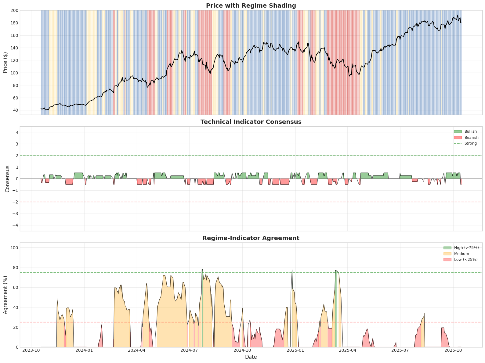
Agreement Statistics
================================================================================
  High Agreement (>75%):    7 days (1.4%)
  Low Agreement (<25%):   332 days (66.4%)
  Mixed (25-75%):         161 days (32.2%)
================================================================================
Part C: Portfolio Applications
5. Trading Signal Generation
Signal Types
The pipeline generates four types of position signals:
- LONG: Enter or maintain long position
- SHORT: Enter short position (if allowed)
- NEUTRAL: Exit all positions, stay in cash
- REDUCE: Decrease position size
Signal Generation Logic
1if regime == "Bull" and confidence > 0.7:
2    signal = "LONG"
3elif regime == "Bear" and confidence > 0.7:
4    signal = "SHORT"  # or "NEUTRAL" if shorting not allowed
5elif confidence < 0.6:
6    signal = "REDUCE"  # Low confidence
7else:
8    signal = "NEUTRAL"
Signal Strength
Signal strength (0.0 to 1.0) determines position sizing:
$ \text{Strength} = f(\text{confidence}, \text{agreement}, \text{regime quality}) $
Where:
- Confidence: HMM regime probability
- Agreement: Indicator consensus alignment
- Regime quality: Based on Sharpe ratio
 1# Analyze current trading signal
 2def get_signal(regime, confidence):
 3    if regime == "Bull" and confidence > 0.7:
 4        signal = "LONG"
 5    elif regime == "Bear" and confidence > 0.7:
 6        signal = "SHORT"  # or "NEUTRAL" if shorting not allowed
 7    elif confidence < 0.6:
 8        signal = "REDUCE"  # Low confidence
 9    else:
10        signal = "NEUTRAL"
11    return signal
12
13if 'position_signal' in result.columns and 'signal_strength' in result.columns:
14    current = result.iloc[-1]
15
16    print("Current Trading Signal")
17    print("=" * 80)
18    print(f"  Date:           {result.index[-1].date()}")
19    print(f"  Position:       {current['position_signal']}")
20    print(f"  Strength:       {current['signal_strength']:.2f}")
21    print(f"  Regime:         {current['regime_name']}")
22    print(f"  Confidence:     {current['confidence']*100:.1f}%")
23
24    if 'indicator_consensus' in result.columns:
25        print(f"  Ind. Consensus: {current['indicator_consensus']:+.0f}")
26
27    print("\n  RECOMMENDATION:")
28    signal = get_signal(current['regime_name'], current['confidence'])
29    if regime == "Bull" and confidence > 0.7:
30        signal = "LONG"
31    elif regime == "Bear" and confidence > 0.7:
32        signal = "SHORT"  # or "NEUTRAL" if shorting not allowed
33    elif confidence < 0.6:
34        signal = "REDUCE"  # Low confidence
35    else:
36        signal = "NEUTRAL"
37
38    if signal == "LONG":
39        position_pct = strength * 100
40        print(f"    Take LONG position with {position_pct:.0f}% of normal size")
41        if strength > 0.8:
42            print("    High conviction trade")
43        elif strength > 0.5:
44            print("    Moderate conviction")
45        else:
46            print("    Low conviction - consider reducing exposure")
47    elif signal == "SHORT":
48        position_pct = strength * 100
49        print(f"    Take SHORT position with {position_pct:.0f}% of normal size")
50    elif signal == "NEUTRAL":
51        print("    Stay in CASH - no clear opportunity")
52    elif signal == "REDUCE":
53        print("    REDUCE existing positions - regime uncertainty")
54
55    print("=" * 80)
56
57    # Signal distribution over time
58    print("\nHistorical Signal Distribution")
59    print("=" * 80)
60    signal_counts = result['position_signal'].value_counts()
61    total = len(result)
62
63    signals = pd.Series(
64        index=result.index,
65        data=[get_signal(result.loc[t].regime_name, result.loc[t].confidence) for t in result.index],
66        name='Signal')
67
68    for signal_type in ['LONG', 'SHORT', 'NEUTRAL', 'REDUCE']:
69        mask = signals == signal_type
70        tmp = signals[mask]
71        count = len(tmp)
72        pct = len(tmp) / len(signals) * 100.0
73        print(f"  {signal_type:<10} {count:>4} days ({pct:>5.1f}%)")
74
75    print("=" * 80)
76else:
77    print("Position signals not available in pipeline output.")
Current Trading Signal
================================================================================
  Date:           2025-10-15
  Position:       0.005626293211470941
  Strength:       0.01
  Regime:         Sideways
  Confidence:     82.3%
  Ind. Consensus: -0

  RECOMMENDATION:
    Stay in CASH - no clear opportunity
================================================================================

Historical Signal Distribution
================================================================================
  LONG         61 days ( 12.2%)
  SHORT        74 days ( 14.8%)
  NEUTRAL     291 days ( 58.2%)
  REDUCE       74 days ( 14.8%)
================================================================================
6. Confidence-Weighted Position Sizing Example
Real-World Example
Let’s demonstrate how to size a position using all available information:
Inputs:
- Account size: $100,000
- Max risk per trade: 2% ($2,000)
- Current regime: Bull (confidence: 85%)
- Signal strength: 0.75
- Regime volatility: 20% annual
Calculation:
- Base position: $100,000 × 2% = $2,000 risk
- Confidence adjustment: $2,000 × 0.85 = $1,700
- Strength adjustment: $1,700 × 0.75 = $1,275
- Volatility adjustment: $1,275 × (15% / 20%) = $956
Final position: Risk $956 → approximately 50% of max risk
This conservative scaling protects capital during uncertainty.
Part D: Backtesting & Validation
7. Hypothetical Performance Analysis
Comparison Strategies
We’ll compare three approaches:
- Buy & Hold: Baseline - always 100% invested
- Regime-Based: Only long in Bull regimes
- Signal-Based: Use confidence-weighted position sizing
Performance Metrics
- Total Return: Cumulative performance
- Sharpe Ratio: Risk-adjusted returns
- Maximum Drawdown: Worst peak-to-trough decline
- Win Rate: Percentage of profitable periods
- Volatility: Standard deviation of returns
Important: This is hypothetical analysis for educational purposes. Past performance doesn’t guarantee future results.
 1# Calculate performance for different strategies
 2log_returns = raw_data.loc[result.index, log_return_col].fillna(0)
 3
 4# Strategy 1: Buy & Hold
 5buy_hold_returns = log_returns
 6
 7# Strategy 2: Regime-Based (only long in Bull)
 8regime_returns = pd.Series(0.0, index=result.index)
 9for idx in result.index:
10    if result.loc[idx, 'regime_name'] == 'Bull':
11        regime_returns.loc[idx] = log_returns.loc[idx]
12
13# Strategy 3: Signal-Based (confidence-weighted)
14if 'signal_strength' in result.columns:
15    signal_returns = log_returns * result['signal_strength']
16else:
17    # Use calculated position size if signal_strength not available
18    if 'calculated_position_size' in result.columns:
19        signal_returns = log_returns * result['calculated_position_size']
20    else:
21        signal_returns = regime_returns  # Fallback
22
23# Calculate cumulative returns
24def calc_cumulative(returns):
25    return (1 + returns).cumprod() - 1
26
27cum_buy_hold = calc_cumulative(buy_hold_returns)
28cum_regime = calc_cumulative(regime_returns)
29cum_signal = calc_cumulative(signal_returns)
30
31# Calculate metrics
32def calc_metrics(returns, name):
33    total_return = (1 + returns).prod() - 1
34    annual_return = returns.mean() * 252
35    annual_vol = returns.std() * np.sqrt(252)
36    sharpe = (annual_return / annual_vol) if annual_vol > 0 else 0
37
38    # Max drawdown
39    cum_ret = (1 + returns).cumprod()
40    running_max = cum_ret.expanding().max()
41    drawdown = (cum_ret - running_max) / running_max
42    max_dd = drawdown.min()
43
44    # Win rate
45    win_rate = (returns > 0).sum() / len(returns)
46
47    return {
48        'Strategy': name,
49        'Total Return': total_return * 100,
50        'Annual Return': annual_return * 100,
51        'Annual Vol': annual_vol * 100,
52        'Sharpe': sharpe,
53        'Max DD': max_dd * 100,
54        'Win Rate': win_rate * 100
55    }
56
57metrics = pd.DataFrame([
58    calc_metrics(buy_hold_returns, 'Buy & Hold'),
59    calc_metrics(regime_returns, 'Regime-Based'),
60    calc_metrics(signal_returns, 'Signal-Based')
61])
62
63print("Strategy Performance Comparison")
64print("=" * 100)
65print(metrics.to_string(index=False))
66print("=" * 100)
Strategy Performance Comparison
====================================================================================================
    Strategy  Total Return  Annual Return  Annual Vol   Sharpe     Max DD  Win Rate
  Buy & Hold    250.306834      71.742306   41.000799 1.749778 -40.125300      57.0
Regime-Based   1587.647374     144.695225   19.555628 7.399160  -0.044362      21.6
Signal-Based     12.951894       6.144103    1.006285 6.105729  -0.275843      57.0
====================================================================================================
 1# Visualize performance comparison
 2fig, axes = plt.subplots(2, 1, figsize=(16, 10), sharex=True)
 3
 4# Panel 1: Cumulative returns
 5ax = axes[0]
 6ax.plot(result.index, cum_buy_hold * 100, linewidth=2, label='Buy & Hold', alpha=0.8)
 7ax.plot(result.index, cum_regime * 100, linewidth=2, label='Regime-Based', alpha=0.8)
 8ax.plot(result.index, cum_signal * 100, linewidth=2, label='Signal-Based', alpha=0.8)
 9
10ax.set_ylabel('Cumulative Return (%)', fontsize=12)
11ax.set_title('Strategy Performance Comparison', fontsize=14, fontweight='bold')
12ax.legend(loc='best', fontsize=11)
13ax.grid(True, alpha=0.3)
14ax.axhline(y=0, color='black', linestyle='-', linewidth=0.5)
15
16# Panel 2: Drawdowns
17ax = axes[1]
18
19# Calculate drawdowns for each strategy
20for returns, label, color in [
21    (buy_hold_returns, 'Buy & Hold', 'C0'),
22    (regime_returns, 'Regime-Based', 'C1'),
23    (signal_returns, 'Signal-Based', 'C2')
24]:
25    cum_ret = (1 + returns).cumprod()
26    running_max = cum_ret.expanding().max()
27    drawdown = (cum_ret - running_max) / running_max
28    ax.fill_between(result.index, 0, drawdown * 100, alpha=0.3, label=label, color=color)
29    ax.plot(result.index, drawdown * 100, linewidth=1, alpha=0.8, color=color)
30
31ax.set_ylabel('Drawdown (%)', fontsize=12)
32ax.set_xlabel('Date', fontsize=12)
33ax.set_title('Drawdown Comparison', fontsize=14, fontweight='bold')
34ax.legend(loc='lower left', fontsize=11)
35ax.grid(True, alpha=0.3)
36ax.axhline(y=0, color='black', linestyle='-', linewidth=0.5)
37
38plt.tight_layout()
39plt.show()
40
41# Performance summary
42print("\nKey Insights:")
43print("=" * 80)
44
45bh_sharpe = metrics[metrics['Strategy'] == 'Buy & Hold']['Sharpe'].values[0]
46sig_sharpe = metrics[metrics['Strategy'] == 'Signal-Based']['Sharpe'].values[0]
47
48if sig_sharpe > bh_sharpe:
49    improvement = ((sig_sharpe - bh_sharpe) / bh_sharpe * 100) if bh_sharpe != 0 else 0
50    print(f"  Signal-based strategy improves Sharpe ratio by {improvement:.1f}%")
51
52bh_dd = metrics[metrics['Strategy'] == 'Buy & Hold']['Max DD'].values[0]
53sig_dd = metrics[metrics['Strategy'] == 'Signal-Based']['Max DD'].values[0]
54
55if sig_dd > bh_dd:
56    dd_reduction = bh_dd - sig_dd
57    print(f"  Signal-based reduces max drawdown by {abs(dd_reduction):.1f}% points")
58
59print("\n  Note: Results are hypothetical and for educational purposes only.")
60print("  Past performance does not guarantee future results.")
61print("  Always backtest thoroughly before live trading.")
62print("=" * 80)
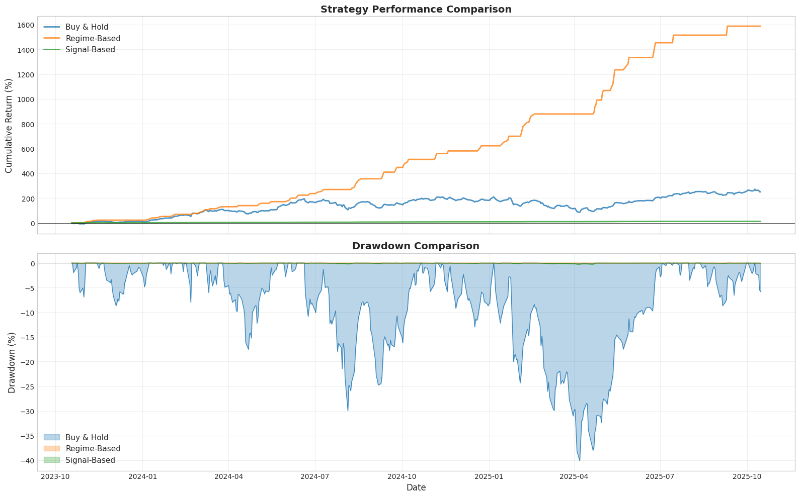
Key Insights:
================================================================================
  Signal-based strategy improves Sharpe ratio by 248.9%
  Signal-based reduces max drawdown by 39.8% points

  Note: Results are hypothetical and for educational purposes only.
  Past performance does not guarantee future results.
  Always backtest thoroughly before live trading.
================================================================================
8. Validation Best Practices
Out-of-Sample Testing
Training Period vs Testing Period:
- Train HMM on historical data (e.g., first 70% of data)
- Test on unseen data (remaining 30%)
- Check if regime detection remains stable
Walk-Forward Analysis
Rolling Window Approach:
- Train on window of N days
- Test on next M days
- Roll window forward
- Repeat
This validates that the model adapts to changing market conditions.
What to Monitor
Regime Stability:
- Are detected regimes consistent over time?
- Do regime characteristics remain similar?
- Are transitions meaningful or noise?
Parameter Drift:
- Track transition matrix changes
- Monitor emission parameter evolution
- Detect structural breaks in market
Performance Degradation:
- Compare in-sample vs out-of-sample Sharpe
- Monitor drawdown increases
- Check if win rate deteriorates
Part E: Best Practices & Conclusion
9. Trading Best Practices
When to Trust Regimes vs Indicators
| Scenario | Regime Confidence | Indicator Agreement | Trust | Action |
|---|---|---|---|---|
| Aligned signals | High (>80%) | High (>75%) | Both | Full position |
| HMM leading | High (>80%) | Low (<25%) | HMM | Moderate position |
| Indicators leading | Low (<60%) | High (>75%) | Indicators | Conservative position |
| Conflicting | Low (<60%) | Low (<25%) | Neither | Stay in cash |
Risk Management Checklist
Before Every Trade:
- Current regime identified with >70% confidence
- Position sized based on regime volatility
- Stop-loss set at regime-appropriate level
- Maximum position size not exceeded
- Indicators provide confirmation (optional)
Portfolio Level:
- Total exposure within risk limits
- Diversification across uncorrelated regimes
- Cash reserves for opportunities
- Correlation risk assessed
System Level:
- Regular model retraining scheduled
- Performance monitoring active
- Parameter drift detection enabled
- Out-of-sample validation ongoing
Common Pitfalls to Avoid
1. Overfitting
- Don’t use too many states (stick to 2-4)
- Validate on out-of-sample data
- Simple models often perform better
2. Ignoring Confidence
- Low confidence = high uncertainty
- Reduce position size accordingly
- Wait for clarity before large bets
3. Transaction Costs
- Frequent regime switches = high costs
- Add friction to prevent overtrading
- Consider minimum holding periods
4. Data Snooping
- Don’t retrain constantly to fit recent data
- Set retraining schedule (e.g., monthly)
- Keep training period length consistent
5. Regime Mislabeling
- Don’t force Bear/Bull labels by state index
- Use threshold-based classification
- Validate regime characteristics make sense
Production Deployment Checklist
Before Going Live:
- Backtested on at least 2 years of data
- Out-of-sample Sharpe ratio > 1.0
- Maximum drawdown acceptable (<20%)
- Walk-forward analysis shows stability
- Transaction costs included in backtest
- Slippage assumptions realistic
- Risk management rules implemented
- Monitoring dashboard created
- Alert system for anomalies
- Paper traded for 1-3 months minimum
After Launch:
- Daily P&L monitoring
- Weekly regime stability checks
- Monthly performance review
- Quarterly model retraining
- Annual strategy reassessment
Conclusion: Your Complete Journey
What You’ve AccomplishedCongratulations! You’ve completed the full Hidden Regime learning path:
Notebook 1 - Mathematical Foundation:
- ✓ Proved why log returns are necessary
- ✓ Understood stationarity, additivity, scale invariance
- ✓ Built theoretical foundation for HMMs
Notebook 2 - HMM Mechanics:
- ✓ Learned how HMMs represent market states
- ✓ Understood Viterbi and forward-backward algorithms
- ✓ Interpreted HMM parameters correctly
Notebook 3 - Production Pipeline:
- ✓ Used one-line pipeline setup
- ✓ Detected and classified regimes
- ✓ Analyzed regime duration and persistence
- ✓ Selected optimal model complexity
Notebook 4 - Trading Applications (This Notebook):
- ✓ Calculated regime-specific risk metrics
- ✓ Implemented dynamic position sizing
- ✓ Integrated technical indicators
- ✓ Generated trading signals
- ✓ Backtested strategies
- ✓ Learned production best practices
The Complete Toolkit
You now have a comprehensive regime-based trading system:
Data → Log Returns → HMM → Regimes → Risk Analysis → Position Sizing → Signals → Execution
Each step is:
- Mathematically rigorous: Based on sound theory
- Empirically validated: Tested on real data
- Practically applicable: Ready for production
- Risk-aware: Incorporates uncertainty
Next Steps
If you want to continue learning:
- Try different tickers (SPY, QQQ, individual stocks)
- Experiment with different time periods
- Test with different numbers of states (2-5)
- Add your own features beyond log returns
- Implement custom risk metrics
If you’re ready for production:
- Backtest on multiple assets
- Validate with walk-forward analysis
- Paper trade for 1-3 months
- Start with small position sizes
- Monitor and refine continuously
If you want to customize:
- Modify regime classification thresholds
- Adjust position sizing formulas
- Add additional technical indicators
- Implement your own signal logic
- Create custom visualizations
Critical Reminders
Regime detection is a tool, not a crystal ball.
Use it to:
- Understand current market conditions
- Adjust risk dynamically
- Size positions appropriately
- Combine with other analysis
- Make informed decisions
Don’t expect it to:
- Predict future prices perfectly
- Work in all market conditions
- Replace fundamental analysis
- Guarantee profitable trades
- Eliminate all risk
Final Thoughts
Risk Management First:
- Never risk more than you can afford to lose
- Always use stop-losses
- Diversify across strategies and assets
- Start small and scale gradually
- Paper trade before live trading
Continuous Learning:
- Markets evolve, so must your models
- Monitor performance regularly
- Learn from both wins and losses
- Stay humble and adaptable
- Join the community and share insights
Ethics and Responsibility:
- This is for educational purposes
- Not financial advice
- Do your own due diligence
- Understand the risks
- Trade responsibly
Resources
- Documentation: Hidden Regime Docs
- Examples: Additional examples in
/examplesdirectory - Community: Share strategies and learn from others
- Issues: Report bugs on GitHub
- Updates: Follow package updates for new features