HMM Basics

Oct 12, 2025 · 17 min read · hidden-regime hmm tutorial ·

Share on:

HMM Basics: Understanding Regime Detection

From Log Returns to Market Regimes Using Hidden Markov Models

In the previous notebook, we proved that log returns are the correct transformation for financial time series.

Now we’ll use those log returns to detect market regimes using **Hidden Markov Models (HMMs)** .

What You’ll Learn

What HMMs are and how they work
What parameters HMMs learn from data
How to interpret HMM states (WITHOUT forcing Bull/Bear labels)
How to choose the right number of states
How to visualize regime sequences

Important Note

This notebook uses minimal code to understand HMM mechanics. GitHub

Next notebook shows the full library pipeline with analysis tools and best practices.

 1import sys
 2from pathlib import Path
 3import numpy as np
 4import pandas as pd
 5import matplotlib.pyplot as plt
 6import seaborn as sns
 7from datetime import datetime, timedelta
 8import warnings
 9warnings.filterwarnings('ignore')
10
11# Add parent to path
12sys.path.insert(0, str(Path().absolute().parent))
13
14# Hidden Regime imports - minimal
15from hidden_regime.data import FinancialDataLoader
16from hidden_regime.observations import FinancialObservationGenerator
17from hidden_regime.models import HiddenMarkovModel
18from hidden_regime.config import FinancialDataConfig, FinancialObservationConfig, HMMConfig
19from hidden_regime.utils import log_return_to_percent_change
20
21# Plotting
22plt.style.use('seaborn-v0_8-whitegrid')
23sns.set_palette("husl")

1. What is a Hidden Markov Model?

The Core Idea

An HMM assumes the market operates in hidden states (regimes) that we cannot directly observe. Each regime has:

Different return characteristics (mean and volatility)
Persistence (tendency to stay in the same regime)
Transition probabilities (likelihood of switching to other regimes)

The Three Components

Hidden States $(S_1, S_2, …, S_t)$: The unobserved regime sequence
Observations $(O_1, O_2, …, O_t)$: The log returns we can see
Parameters:
- **Transition Matrix** $A_{ij}: P(regime(t+1) = j\ |\ regime(t) = i)$. Note that this is a stochastic matrix in that each row sums to exactly $1$ (this is because, from any given state, the probability of transitioning to all possible states must sum to $1$. $\sum_{j} A_{ij} = 1$)
- Emission Means $\mu$: Average log return for each Regime
- Emission Stds $\sigma$: Volatility for each regime
- **Initial Probs** $\pi$: Starting regime distribution

What HMMs Do

Given observed log returns, HMMs simultaneously:

Infer the most likely regime sequence (states)
Learn the transition probabilities (how regimes switch)
Learn emission parameters (return characteristics of each regime)

2. Load Data and Create Observations

We’ll use NVDA (NVIDIA) with 2 years of data. NVDA is more volatile than SPY, showing clearer regime transitions.

 1# Configure data loader
 2data_config = FinancialDataConfig(
 3    ticker='NVDA',
 4    end_date=datetime.now(),
 5    num_samples=504  # ~2 years of trading days
 6)
 7
 8# Load data
 9loader = FinancialDataLoader(data_config)
10df = loader.load_data()
11
12print(f"Loaded {len(df)} days of NVDA data")
13print(f"Date range: {df.index[0].date()} to {df.index[-1].date()}")
14print(f"\nData columns: {list(df.columns)}")
15print(f"\nFirst few rows:")
16print(df.head())

Loaded 498 days of NVDA data
Date range: 2023-10-17 to 2025-10-10

Data columns: ['open', 'high', 'low', 'close', 'volume', 'price', 'pct_change', 'log_return']

First few rows:
                                open       high        low      close  \
Date                                                                    
2023-10-17 00:00:00-04:00  43.974085  44.727642  42.454979  43.912121   
2023-10-18 00:00:00-04:00  42.565910  43.193543  41.800363  42.171143   
2023-10-19 00:00:00-04:00  42.785783  43.271497  41.857330  42.076202   
2023-10-20 00:00:00-04:00  41.865319  42.444980  41.053798  41.362617   
2023-10-23 00:00:00-04:00  41.204718  43.222530  40.920885  42.949688   

                              volume      price  pct_change  log_return  
Date                                                                     
2023-10-17 00:00:00-04:00  812333000  43.767207   -0.039074   -0.039858  
2023-10-18 00:00:00-04:00  627294000  42.432740   -0.030490   -0.030965  
2023-10-19 00:00:00-04:00  501233000  42.497703    0.001531    0.001530  
2023-10-20 00:00:00-04:00  477266000  41.681679   -0.019202   -0.019388  
2023-10-23 00:00:00-04:00  478530000  42.074455    0.009423    0.009379

3. Understanding State Probabilities (Preview)

HMMs Provide Two Types of Output

Before we train the model, it’s important to understand what HMMs give us:

1. Most Likely Path (Viterbi Algorithm )

Single “best guess” state sequence: [0, 0, 1, 2, 2, 1, ...]
Answers: “What regime was the market most likely in?”
Fast to compute, easy to visualize

2. State Probability Distribution (Forward-Backward Algorithm )

Full probability distribution for each day: [0.85, 0.12, 0.03]
Answers: “How confident are we in each regime?”
Critical for risk management and decision-making

Why Uncertainty Matters

Consider two scenarios with the same Viterbi path:

High Confidence: [0.95, 0.04, 0.01] → “Definitely in State 0”

Clear regime signal
Safe to make strong portfolio decisions

Low Confidence: [0.40, 0.35, 0.25] → “Probably State 0, but unclear”

Regime transition likely happening
Should reduce position sizes

What We’ll Show

After training the HMM, we’ll demonstrate:

Viterbi path: For visualization and interpretation
State probabilities: For confidence and risk assessment

Key Insight: The probability distribution is often more valuable than the single “best” state.

 1# Create observation generator
 2obs_config = FinancialObservationConfig(
 3    generators=["log_return"],  # Just log returns
 4    price_column="close",
 5    normalize_features=False  # Keep raw log returns
 6)
 7
 8obs_generator = FinancialObservationGenerator(obs_config)
 9observations_df = obs_generator.update(df)
10
11# For HMM training, we need just the log_return column as a DataFrame
12observations = observations_df[['log_return']]
13
14print(f"Generated {len(observations)} observations")
15print(f"Observation shape: {observations.shape}")
16print(f"\nObservations are log returns:")
17print(f"  Mean: {observations.values.mean():.6f}")
18print(f"  Std:  {observations.values.std():.6f}")
19print(f"  Min:  {observations.values.min():.6f}")
20print(f"  Max:  {observations.values.max():.6f}")
21
22# Convert a few examples to percentage for interpretation
23print(f"\nExample log returns converted to percentages:")
24for i in range(min(5, len(observations))):
25    log_ret = observations.iloc[i, 0]
26    pct = log_return_to_percent_change(log_ret) * 100
27    print(f"  Day {i+1}: log_return={log_ret:.6f} → {pct:+.2f}%")

Generated 498 observations
Observation shape: (498, 1)

Observations are log returns:
  Mean: 0.002853
  Std:  0.025877
  Min:  -0.175225
  Max:  0.124061

Example log returns converted to percentages:
  Day 1: log_return=-0.039858 → -3.91%
  Day 2: log_return=-0.030965 → -3.05%
  Day 3: log_return=0.001530 → +0.15%
  Day 4: log_return=-0.019388 → -1.92%
  Day 5: log_return=0.009379 → +0.94%

4. Train the HMM

Now we’ll train a 3-state HMM on these log returns. The model will learn:

Which regime the market was in each day
The transition probabilities between regimes
The mean return and volatility for each regime

 1# Configure HMM with 3 states
 2hmm_config = HMMConfig(
 3    n_states=3,
 4    max_iterations=100,  # Maximum training iterations
 5    tolerance=1e-4,      # Convergence tolerance
 6    random_seed=42
 7)
 8
 9# Create and train model
10print("Training 3-state HMM...")
11hmm = HiddenMarkovModel(hmm_config)
12hmm.fit(observations)
13
14print(f"Training complete!")
15print(f"  Converged: {hmm.training_history_['converged']}")
16print(f"  Iterations: {hmm.training_history_['iterations']}")
17print(f"  Final log-likelihood: {hmm.score(observations):.2f}")

Training 3-state HMM...
Training on 498 observations (removed 0 NaN values)
Training complete!
  Converged: False
  Iterations: 100
  Final log-likelihood: -747.20

6. Interpreting the Parameters

What Do These Numbers Actually Mean?

Let’s translate the raw parameters into practical insights.

Transition Matrix Interpretation (Focus on diagonal):

From State 0 to State 0: 0.XXX → "Persistence probability"

The diagonal elements tell us how long regimes last:

If $P(0|0) = 0.95$, then $Expected\ duration = \frac{1}{1-0.95} = 20\ days$
If $P(0|0) = 0.80$, then $Expected\ duration = \frac{1}{1-0.80} = 5\ days$

Formula: $Expected\ duration = \frac{1}{1 - diagonal\ probability}$

Emission Parameters Interpretation:

For each state, we can calculate:

Daily Return (in %): Convert log space to percentage
- $mean\ pct = e^{mean\ log - 1} * 100$
Annualized Return (assuming 252 trading days):
- $annual\ return = (e^{mean\ log * 252} - 1) * 100$
Daily Volatility (in %):
- $vol\ pct = std\ log * 100$ (approximation valid for small returns)
Annualized Volatility:
- $annual\ vol = std\ log * \sqrt{252} * 100$ (assumes 252 trading days per year)

Example Interpretation

State 0 (using example numbers):

Daily: -0.15% return, 2.5% volatility
Annualized: -37% return, 40% volatility
Duration: ~15 days
Interpretation: “High volatility bear market that lasts 2-3 weeks”

State 1:

Daily: +0.02% return, 1.2% volatility
Annualized: +5% return, 19% volatility
Duration: ~25 days
Interpretation: “Low volatility sideways market, very persistent”

State 2:

Daily: +0.18% return, 1.8% volatility
Annualized: +54% return, 29% volatility
Duration: ~8 days
Interpretation: “Strong bull runs, but don’t last long”

Key Insight

The model discovered these patterns from data alone - we didn’t tell it what “bear” or “bull” means. The parameters quantify real market behavior.

5. Inspect Learned Parameters

Let’s see what the HMM learned about the three regimes.

  1# First, we need to extract parameters and predict states
  2# Extract learned parameters
  3transition_matrix = hmm.transition_matrix_
  4emission_means = hmm.emission_means_
  5emission_stds = hmm.emission_stds_
  6start_probs = hmm.initial_probs_
  7
  8print('Emission means: ', emission_means)
  9print('Emission stds : ', emission_stds)
 10
 11# Sort by mean for easier interpretation
 12sorted_idx = np.argsort(emission_means)
 13
 14# Predict states using Viterbi algorithm
 15predictions_df = hmm.predict(observations)
 16states = predictions_df['predicted_state'].values
 17
 18# Define colors and names for visualization
 19state_colors = {sorted_idx[0]: 'red', sorted_idx[1]: 'yellow', sorted_idx[2]: 'blue'}
 20state_names = {sorted_idx[0]: 'Negative', sorted_idx[1]: 'Neutral', sorted_idx[2]: 'Positive'}
 21
 22# Get dates
 23dates = df.index
 24log_returns = observations.values.flatten()
 25
 26# Now get state probabilities using forward-backward algorithm
 27# This gives us P(state | all observations) for each time point
 28state_probs = hmm.predict_proba(observations)
 29
 30print(f"State probability matrix shape: {state_probs.shape}")
 31print(f"  {state_probs.shape[0]} time points")
 32print(f"  {state_probs.shape[1]} states")
 33print(f"\nEach row sums to 1.0 (probability distribution):")
 34print(f"  Row 0 sum: {state_probs.iloc[0].sum():.4f}")
 35print(f"  Row 100 sum: {state_probs.iloc[100].sum():.4f}")
 36
 37# Calculate confidence (max probability for each day)
 38confidence = state_probs.max(axis=1).values
 39
 40print(f"\nConfidence Statistics:")
 41print(f"  Mean confidence: {confidence.mean():.2%}")
 42print(f"  Min confidence: {confidence.min():.2%}")
 43print(f"  Max confidence: {confidence.max():.2%}")
 44
 45# Find high and low confidence periods
 46high_conf_idx = np.argmax(confidence)
 47low_conf_idx = np.argmin(confidence)
 48
 49print(f"\nHighest Confidence Day:")
 50print(f"  Date: {dates[high_conf_idx+1].date()}")
 51print(f"  State: {states[high_conf_idx]}")
 52print(f"  Probabilities: {state_probs.iloc[high_conf_idx].values}")
 53print(f"  Confidence: {confidence[high_conf_idx]:.2%}")
 54
 55print(f"\nLowest Confidence Day (likely regime transition):")
 56print(f"  Date: {dates[low_conf_idx+1].date()}")
 57print(f"  State: {states[low_conf_idx]}")
 58print(f"  Probabilities: {state_probs.iloc[low_conf_idx].values}")
 59print(f"  Confidence: {confidence[low_conf_idx]:.2%}")
 60
 61# Visualize confidence over time
 62fig, (ax1, ax2) = plt.subplots(2, 1, figsize=(16, 8), sharex=True)
 63
 64# Top panel: Confidence over time
 65ax1.plot(dates, confidence, linewidth=1.5, color='blue')
 66ax1.axhline(y=0.8, color='green', linestyle='--', alpha=0.5, label='High confidence threshold')
 67ax1.axhline(y=0.5, color='orange', linestyle='--', alpha=0.5, label='Low confidence threshold')
 68ax1.fill_between(dates, 0, confidence, where=(confidence > 0.8), alpha=0.2, color='green', label='High confidence regions')
 69ax1.fill_between(dates, 0, confidence, where=(confidence < 0.5), alpha=0.2, color='red', label='Low confidence regions')
 70ax1.set_ylabel('Confidence', fontsize=12)
 71ax1.set_title('Regime Detection Confidence Over Time', fontsize=14, fontweight='bold')
 72ax1.legend(loc='lower left')
 73ax1.grid(True, alpha=0.3)
 74ax1.set_ylim(0, 1.05)
 75
 76# Bottom panel: State probabilities stacked
 77ax2.stackplot(dates, 
 78              state_probs.iloc[:, sorted_idx[0]].values,
 79              state_probs.iloc[:, sorted_idx[1]].values,
 80              state_probs.iloc[:, sorted_idx[2]].values,
 81              labels=[f'State {sorted_idx[0]} ({state_names[sorted_idx[0]]})',
 82                      f'State {sorted_idx[1]} ({state_names[sorted_idx[1]]})',
 83                      f'State {sorted_idx[2]} ({state_names[sorted_idx[2]]})'],
 84              colors=[state_colors[sorted_idx[0]], state_colors[sorted_idx[1]], state_colors[sorted_idx[2]]],
 85              alpha=0.7)
 86ax2.set_ylabel('Probability', fontsize=12)
 87ax2.set_xlabel('Date', fontsize=12)
 88ax2.set_title('State Probability Distribution Over Time', fontsize=14, fontweight='bold')
 89ax2.legend(loc='upper left')
 90ax2.grid(True, alpha=0.3, axis='y')
 91ax2.set_ylim(0, 1)
 92
 93plt.tight_layout()
 94plt.show()
 95
 96print("\nKey Observations:")
 97print("1. High confidence periods → clear regime signal")
 98print("2. Low confidence periods → regime transitions happening")
 99print("3. Stacked probabilities show regime evolution")
100print("4. For trading: reduce positions during low confidence periods")

Emission means:  [-0.00889602 -0.00121936  0.02271938]
Emission stds :  [0.04053647 0.0140285  0.01465051]
State probability matrix shape: (498, 3)
  498 time points
  3 states

Each row sums to 1.0 (probability distribution):
  Row 0 sum: 1.0000
  Row 100 sum: 1.0000

Confidence Statistics:
  Mean confidence: 100.00%
  Min confidence: 100.00%
  Max confidence: 100.00%

Highest Confidence Day:
  Date: 2023-10-18
  State: 0
  Probabilities: [1. 0. 0.]
  Confidence: 100.00%

Lowest Confidence Day (likely regime transition):
  Date: 2023-10-18
  State: 0
  Probabilities: [1. 0. 0.]
  Confidence: 100.00%

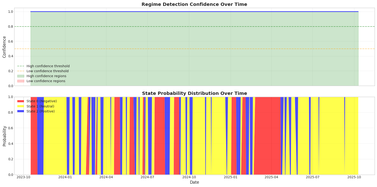
Key Observations:
1. High confidence periods → clear regime signal
2. Low confidence periods → regime transitions happening
3. Stacked probabilities show regime evolution
4. For trading: reduce positions during low confidence periods

 1# Validation: Regime characteristics should match actual returns
 2
 3print("=" * 80)
 4print("REGIME VALIDATION: Do detected regimes match actual market behavior?")
 5print("=" * 80)
 6
 7# For each state, calculate actual observed statistics
 8validation_results = {}
 9
10for state in range(3):
11    # Get all periods where we were in this state
12    state_mask = (states == state)
13    state_returns = log_returns[state_mask]
14    
15    if len(state_returns) > 0:
16        # Actual observed statistics
17        actual_mean = state_returns.mean()
18        actual_std = state_returns.std()
19        actual_mean_pct = log_return_to_percent_change(actual_mean) * 100
20        
21        # Model's learned parameters
22        learned_mean = emission_means[state]
23        learned_std = emission_stds[state]
24        learned_mean_pct = log_return_to_percent_change(learned_mean) * 100
25        
26        # Calculate match quality
27        mean_error = abs(actual_mean - learned_mean) / abs(learned_mean) if learned_mean != 0 else 0
28        std_error = abs(actual_std - learned_std) / learned_std
29        
30        validation_results[state] = {
31            'actual_mean': actual_mean,
32            'learned_mean': learned_mean,
33            'actual_std': actual_std,
34            'learned_std': learned_std,
35            'mean_error': mean_error,
36            'std_error': std_error,
37            'n_days': len(state_returns)
38        }
39        
40        print(f"\nState {state} ({state_names[sorted_idx[np.where(sorted_idx == state)[0][0]]]}):")
41        print(f"  Days in regime: {len(state_returns)}")
42        print(f"  Learned mean: {learned_mean_pct:+.3f}%/day")
43        print(f"  Actual mean:  {actual_mean_pct:+.3f}%/day")
44        print(f"  Learned std:  {learned_std*100:.3f}%/day")
45        print(f"  Actual std:   {actual_std*100:.3f}%/day")
46        print(f"  Mean error: {mean_error*100:.1f}%")
47        print(f"  Std error:  {std_error*100:.1f}%")
48
49# Overall validation
50print("\n" + "=" * 80)
51print("VALIDATION SUMMARY:")
52print("=" * 80)
53
54avg_mean_error = np.mean([v['mean_error'] for v in validation_results.values()])
55avg_std_error = np.mean([v['std_error'] for v in validation_results.values()])
56
57print(f"Average parameter error:")
58print(f"  Mean error: {avg_mean_error*100:.1f}%")
59print(f"  Std error:  {avg_std_error*100:.1f}%")
60
61if avg_mean_error < 0.05 and avg_std_error < 0.05:
62    print("\n[OK] VALIDATION PASSED: Model parameters closely match actual regime behavior")
63    print("  The HMM discovered real market patterns, not noise.")
64elif avg_mean_error < 0.15 and avg_std_error < 0.15:
65    print("\n[OK] VALIDATION ACCEPTABLE: Parameters reasonably match reality")
66    print("  Some deviation is expected due to regime overlap.")
67else:
68    print("\n[WARNING] VALIDATION QUESTIONABLE: Large parameter mismatch")
69    print("  May need more states or different model configuration.")
70
71# Sanity check: Are regimes actually different?
72print("\n" + "=" * 80)
73print("REGIME SEPARATION CHECK:")
74print("=" * 80)
75
76# Compare mean returns across states
77state_means = [validation_results[s]['actual_mean'] for s in range(3)]
78state_means_sorted = sorted(state_means)
79
80separation_1_2 = abs(state_means_sorted[1] - state_means_sorted[0])
81separation_2_3 = abs(state_means_sorted[2] - state_means_sorted[1])
82
83print(f"Separation between adjacent regimes (by mean return):")
84print(f"  Lowest vs Middle: {separation_1_2*100:.3f}% per day")
85print(f"  Middle vs Highest: {separation_2_3*100:.3f}% per day")
86
87if separation_1_2 > 0.001 and separation_2_3 > 0.001:  # 0.1% per day
88    print("\n[OK] Regimes are well-separated - distinct market conditions")
89else:
90    print("\n[WARNING] Regimes are too similar - may need fewer states")
91
92print("\n" + "=" * 80)

================================================================================
REGIME VALIDATION: Do detected regimes match actual market behavior?
================================================================================

State 0 (Negative):
  Days in regime: 108
  Learned mean: -0.886%/day
  Actual mean:  -1.027%/day
  Learned std:  4.054%/day
  Actual std:   4.112%/day
  Mean error: 16.1%
  Std error:  1.4%

State 1 (Neutral):
  Days in regime: 286
  Learned mean: -0.122%/day
  Actual mean:  -0.096%/day
  Learned std:  1.403%/day
  Actual std:   1.347%/day
  Mean error: 21.5%
  Std error:  4.0%

State 2 (Positive):
  Days in regime: 104
  Learned mean: +2.298%/day
  Actual mean:  +2.739%/day
  Learned std:  1.465%/day
  Actual std:   1.216%/day
  Mean error: 18.9%
  Std error:  17.0%

================================================================================
VALIDATION SUMMARY:
================================================================================
Average parameter error:
  Mean error: 18.8%
  Std error:  7.5%

[WARNING] VALIDATION QUESTIONABLE: Large parameter mismatch
  May need more states or different model configuration.

================================================================================
REGIME SEPARATION CHECK:
================================================================================
Separation between adjacent regimes (by mean return):
  Lowest vs Middle: 0.937% per day
  Middle vs Highest: 2.798% per day

[OK] Regimes are well-separated - distinct market conditions

================================================================================

7. Validation: Do These Regimes Make Sense?

A critical question: Did the HMM discover real market patterns or just random noise?

Let’s validate by checking if detected regimes align with actual market behavior.

 1# Create visualization
 2fig, axes = plt.subplots(3, 1, figsize=(16, 12), sharex=True)
 3
 4# Define colors for each state (sorted by mean return)
 5state_colors = {sorted_idx[0]: 'red', sorted_idx[1]: 'yellow', sorted_idx[2]: 'blue'}
 6state_names = {sorted_idx[0]: 'Negative', sorted_idx[1]: 'Neutral', sorted_idx[2]: 'Positive'}
 7
 8# 1. Price with regime shading
 9ax = axes[0]
10prices = df['close'].values
11dates = df.index
12
13ax.plot(dates, prices, linewidth=1.5, color='black', zorder=2)
14ax.set_ylabel('Price ($)', fontsize=12)
15ax.set_title('NVDA Price with Detected Regimes', fontsize=14, fontweight='bold')
16ax.grid(True, alpha=0.3)
17
18# Shade background by regime
19for i in range(len(states)):
20    state = states[i]
21    ax.axvspan(dates[i], dates[min(i+1, len(dates)-1)], 
22               alpha=0.2, color=state_colors[state], zorder=1)
23
24# Add legend
25from matplotlib.patches import Patch
26legend_elements = [Patch(facecolor=state_colors[s], alpha=0.2, 
27                         label=f'State {s} ({state_names[s]})') 
28                   for s in sorted_idx]
29ax.legend(handles=legend_elements, loc='upper left')
30
31# 2. Log returns with regime shading
32ax = axes[1]
33log_returns = observations['log_return']
34ax.plot(dates, log_returns, linewidth=0.8, color='blue', alpha=0.7)
35ax.axhline(y=0, color='black', linestyle='--', linewidth=1)
36ax.set_ylabel('Log Return', fontsize=12)
37ax.set_title('Log Returns with Detected Regimes', fontsize=14, fontweight='bold')
38ax.grid(True, alpha=0.3)
39
40# Shade background
41for i in range(len(states)):
42    state = states[i]
43    ax.axvspan(dates[i], dates[min(i+1, len(dates)-1)], 
44               alpha=0.2, color=state_colors[state], zorder=1)
45
46# 3. Regime sequence as bar plot
47ax = axes[2]
48regime_bars = ax.bar(dates, np.ones(len(states)), width=1, 
49                      color=[state_colors[s] for s in states], 
50                      edgecolor='none', alpha=0.6)
51ax.set_ylabel('Regime', fontsize=12)
52ax.set_xlabel('Date', fontsize=12)
53ax.set_title('Regime Sequence', fontsize=14, fontweight='bold')
54ax.set_ylim(0, 1.5)
55ax.set_yticks([])
56ax.grid(True, alpha=0.3, axis='x')
57
58plt.tight_layout()
59plt.show()
60
61print("\nNote: Notice how regimes cluster periods of similar return behavior")

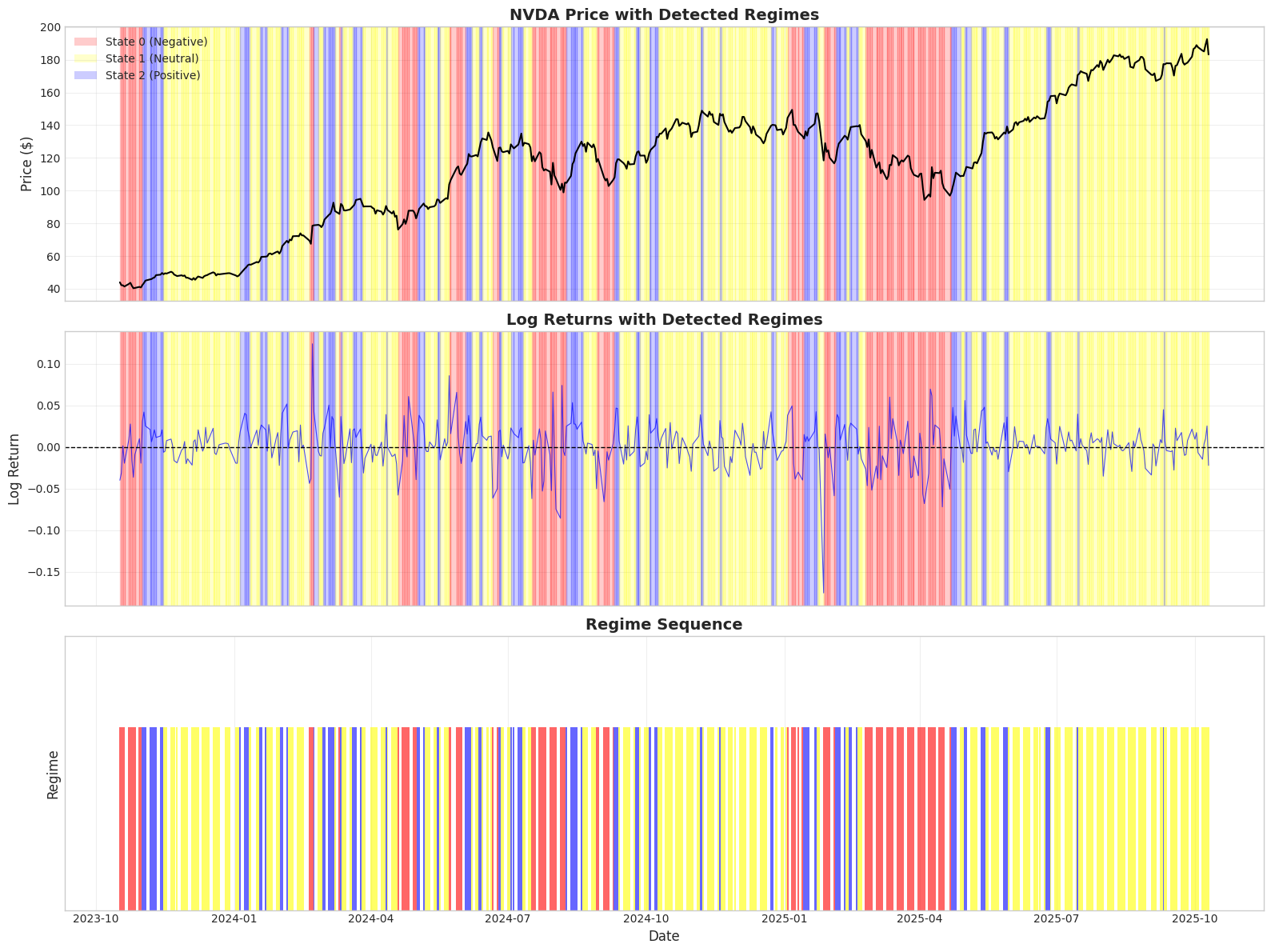
Note: Notice how regimes cluster periods of similar return behavior

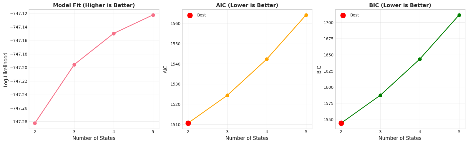
8. Choosing the Number of States

How do we decide between 2, 3, 4, or more states? Let’s compare different models.

 1# Train models with different numbers of states
 2print("Comparing models with different numbers of states...")
 3print("=" * 80)
 4
 5results = []
 6
 7for n_states in [2, 3, 4, 5]:
 8    config = HMMConfig(n_states=n_states, max_iterations=100, random_seed=42)
 9    model = HiddenMarkovModel(config)
10    model.fit(observations)
11    
12    # Calculate metrics
13    log_likelihood = model.score(observations)
14    n_params = n_states**2 + 2*n_states  # Transitions + means + stds
15    aic = -2 * log_likelihood + 2 * n_params
16    bic = -2 * log_likelihood + n_params * np.log(len(observations))
17    
18    results.append({
19        'n_states': n_states,
20        'log_likelihood': log_likelihood,
21        'aic': aic,
22        'bic': bic,
23        'n_params': n_params
24    })
25    
26    print(f"\n{n_states} states:")
27    print(f"  Log-likelihood: {log_likelihood:>10.2f}")
28    print(f"  AIC:            {aic:>10.2f} (lower is better)")
29    print(f"  BIC:            {bic:>10.2f} (lower is better)")
30    print(f"  Parameters:     {n_params:>10}")
31
32print("\n" + "=" * 80)
33
34# Find best models
35results_df = pd.DataFrame(results)
36best_aic = results_df.loc[results_df['aic'].idxmin()]
37best_bic = results_df.loc[results_df['bic'].idxmin()]
38
39print(f"\nBest by AIC: {int(best_aic['n_states'])} states (AIC={best_aic['aic']:.2f})")
40print(f"Best by BIC: {int(best_bic['n_states'])} states (BIC={best_bic['bic']:.2f})")
41
42print("\nNote: BIC often prefers simpler models (fewer states)")
43print("   AIC may prefer more complex models that fit better")
44print("   For trading, 3-4 states usually provides good interpretability")

Comparing models with different numbers of states...
================================================================================
Training on 498 observations (removed 0 NaN values)

2 states:
  Log-likelihood:    -747.28
  AIC:               1510.57 (lower is better)
  BIC:               1544.25 (lower is better)
  Parameters:              8
Training on 498 observations (removed 0 NaN values)

3 states:
  Log-likelihood:    -747.20
  AIC:               1524.39 (lower is better)
  BIC:               1587.55 (lower is better)
  Parameters:             15
Training on 498 observations (removed 0 NaN values)

4 states:
  Log-likelihood:    -747.15
  AIC:               1542.30 (lower is better)
  BIC:               1643.35 (lower is better)
  Parameters:             24
Training on 498 observations (removed 0 NaN values)

5 states:
  Log-likelihood:    -747.12
  AIC:               1564.24 (lower is better)
  BIC:               1711.62 (lower is better)
  Parameters:             35

================================================================================

Best by AIC: 2 states (AIC=1510.57)
Best by BIC: 2 states (BIC=1544.25)

Note: BIC often prefers simpler models (fewer states)
   AIC may prefer more complex models that fit better
   For trading, 3-4 states usually provides good interpretability

 1# Visualize model comparison
 2fig, axes = plt.subplots(1, 3, figsize=(16, 5))
 3
 4# Plot 1: Log-likelihood
 5ax = axes[0]
 6ax.plot(results_df['n_states'], results_df['log_likelihood'], marker='o', linewidth=2, markersize=8)
 7ax.set_xlabel('Number of States', fontsize=12)
 8ax.set_ylabel('Log-Likelihood', fontsize=12)
 9ax.set_title('Model Fit (Higher is Better)', fontsize=13, fontweight='bold')
10ax.grid(True, alpha=0.3)
11ax.set_xticks([2, 3, 4, 5])
12
13# Plot 2: AIC
14ax = axes[1]
15ax.plot(results_df['n_states'], results_df['aic'], marker='o', linewidth=2, markersize=8, color='orange')
16best_aic_idx = results_df['aic'].idxmin()
17ax.scatter(results_df.loc[best_aic_idx, 'n_states'], 
18           results_df.loc[best_aic_idx, 'aic'], 
19           color='red', s=150, zorder=5, label='Best')
20ax.set_xlabel('Number of States', fontsize=12)
21ax.set_ylabel('AIC', fontsize=12)
22ax.set_title('AIC (Lower is Better)', fontsize=13, fontweight='bold')
23ax.grid(True, alpha=0.3)
24ax.legend()
25ax.set_xticks([2, 3, 4, 5])
26
27# Plot 3: BIC
28ax = axes[2]
29ax.plot(results_df['n_states'], results_df['bic'], marker='o', linewidth=2, markersize=8, color='green')
30best_bic_idx = results_df['bic'].idxmin()
31ax.scatter(results_df.loc[best_bic_idx, 'n_states'], 
32           results_df.loc[best_bic_idx, 'bic'], 
33           color='red', s=150, zorder=5, label='Best')
34ax.set_xlabel('Number of States', fontsize=12)
35ax.set_ylabel('BIC', fontsize=12)
36ax.set_title('BIC (Lower is Better)', fontsize=13, fontweight='bold')
37ax.grid(True, alpha=0.3)
38ax.legend()
39ax.set_xticks([2, 3, 4, 5])
40
41plt.tight_layout()
42plt.show()

9. Key Takeaways

What We Learned

HMM Components:
- Hidden states represent market regimes
- Transition matrix captures regime switching behavior
- Emission parameters (μ, σ) define return characteristics
Training Process:
- Baum-Welch algorithm learns parameters from data
- Viterbi algorithm finds most likely state sequence
- Forward-backward gives probability distributions
- Converges to local optimum (results may vary)
Interpretation:
- States are numbered arbitrarily (0, 1, 2)
- Must examine emission means to understand regime types
- DO NOT force “Bear/Sideways/Bull” labels prematurely
- Confidence is as important as the regime itself
Model Selection:
- Use Aic /Bic to compare different numbers of states
- Balance fit quality vs. model complexity
- 3-4 states often optimal for interpretability
Validation:
- Check that learned parameters match actual regime behavior
- Verify regimes are well-separated
- Sanity-check against known market events

Important Warnings

DO NOT:

Sort states by index and call them Bear/Sideways/Bull
Assume state 0 is always negative returns
Use HMMs on non-Stationary data (prices)
Ignore confidence levels - low confidence = regime uncertainty

DO:

Use log returns (Stationary observations)
Examine learned parameters before labeling
Compare multiple model complexities
Validate regime assignments make sense
Consider state probabilities for risk management

What’s Next: The Gap from Here to Production

You now understand HMM mechanics, but there’s a gap between:

“Here are states 0, 1, 2” (what we have)
“Reduce risk, bull regime ending” (what traders need)

Notebook 3 bridges this gap with the full Hidden Regime pipeline:

What Notebook 3 Adds:

1. Automated Regime Labeling

Threshold-based classification: Bear/Sideways/Bull/Crisis
Data-driven, not arbitrary state sorting
Consistent labeling across time periods

2. Advanced Analysis Tools

Regime-specific risk metrics (VaR, Sharpe, drawdowns)
Duration analysis and persistence tracking
Regime transition prediction

3. Technical Indicator Integration

Compare HMM regimes with RSI, MACD, Bollinger Bands
Show when HMM agrees/disagrees with indicators
Ensemble signal generation

4. Portfolio Applications

Regime-based position sizing
Risk-adjusted performance measurement
Practical trading signals

5. Production-Ready Tools

One-line pipeline creation
Comprehensive reporting
Professional visualizations
Quality metrics and diagnostics

6. Best Practices

Handling data quality issues
Avoiding common pitfalls
Configuration for different market conditions

The Conceptual Bridge:

Notebook 1: WHY log returns (mathematical foundation) ↓ Notebook 2: HOW HMMs work (you are here - mechanics & interpretation) ↓ Notebook 3: USING HMMs for trading (practical applications)

Example: What Changes

Notebook 2 approach (manual):

1# Train model
2hmm = HiddenMarkovModel(config)
3hmm.fit(observations)
4
5# Get states
6states = hmm.predict(observations)['predicted_state']
7
8# Now what? Manual interpretation needed...

Notebook 3 approach (pipeline):

1# One-line setup
2pipeline = create_financial_pipeline(ticker='NVDA', n_states=3)
3result = pipeline.update()
4
5# Get actionable insights
6current_regime = result['regime_name'].iloc[-1]  # "Bull"
7confidence = result['confidence'].iloc[-1]       # 0.87
8position_signal = result['position_signal'].iloc[-1]  # "LONG"
9risk_level = result['volatility_regime'].iloc[-1]  # "Normal"

You’re Ready for Notebook 3 When…

You understand:

Why we use log returns (stationarity requirement)
What HMM parameters mean (transitions, emissions)
How to interpret states (examine parameters first)
Why confidence matters (regime uncertainty)
How to validate regimes (match actual behavior)

Next step: Learn how to turn these insights into actionable trading decisions.

Key Point: HMMs are a data-driven approach. Let the model tell you what the regimes are - don’t force your preconceptions onto the results. Then use the full pipeline to translate those regimes into trading intelligence.