HMM 101
HMM 101
An example of how we’ll be using our Hidden Markov Models in this project.
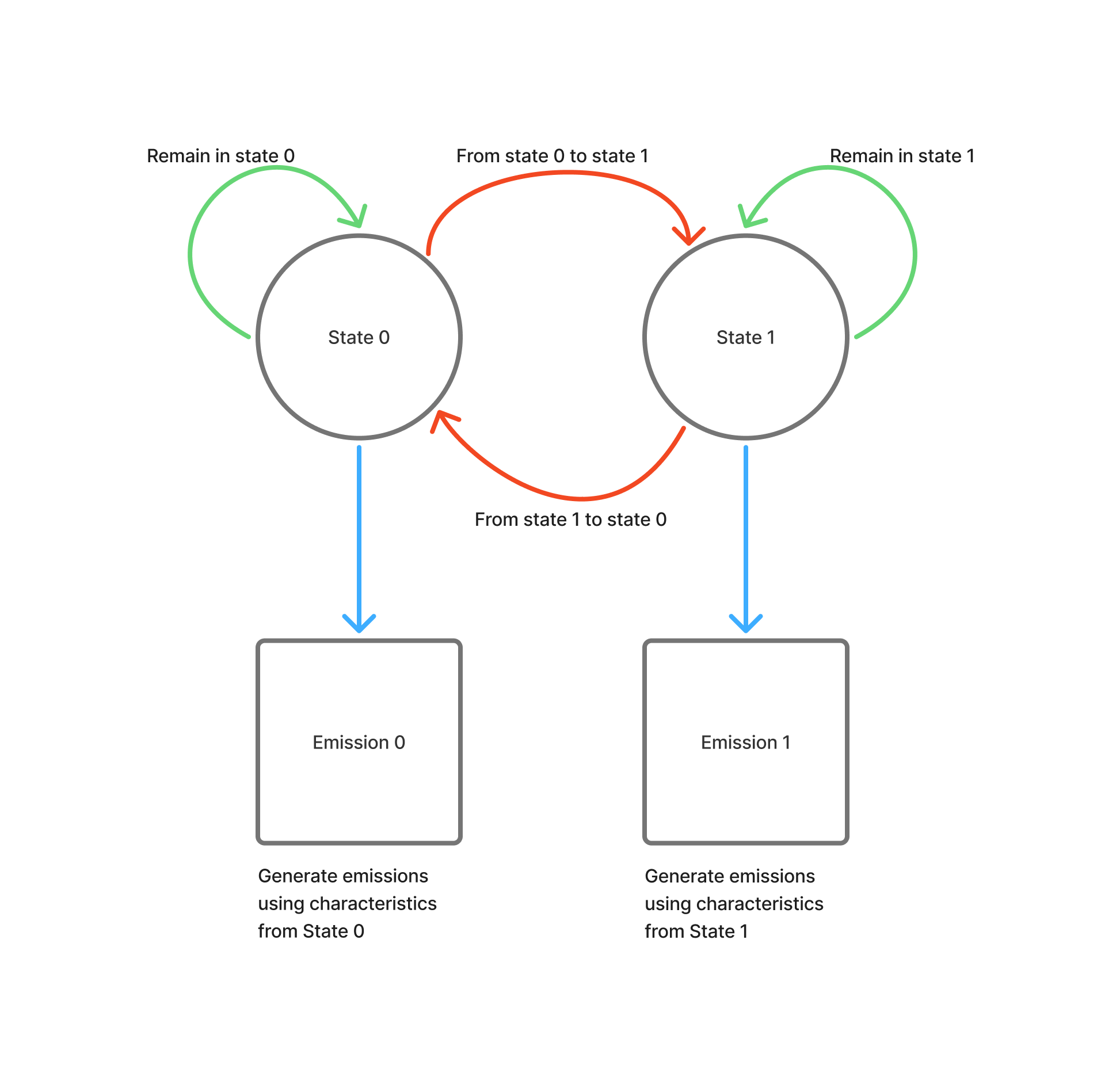
HMM Workflow:
- Initialization (k-means): Cluster observations to get initial emission parameters
- Training (Baum-Welch ): Refine transition matrix & emission distributions
- Prediction (Viterbi ): Decode the most likely state sequence
This notebook can be found on GitHub.
Imports and Setup
 1from datetime import datetime
 2import sys
 3import os
 4from typing import List, Tuple
 5import warnings
 6warnings.filterwarnings('ignore')
 7
 8import numpy as np
 9import matplotlib
10import matplotlib.pyplot as plt
11import pandas as pd
12from sklearn.metrics import accuracy_score, classification_report
13np.random.seed(42) # for repeatability
Hidden Regime Setup
 1# Add the project root to the path
 2sys.path.insert(0, os.path.join(os.path.dirname(os.getcwd()), '..'))
 3
 4# Import HR Model and Config
 5import hidden_regime as hr
 6from hidden_regime.config.model import HMMConfig
 7from hidden_regime.models.hmm import HiddenMarkovModel as HMM
 8
 9# Observations
10from hidden_regime.config.observation import ObservationConfig
11from hidden_regime.observations import BaseObservationGenerator
Problem Statement
We’re going to create a signal that belongs to one of N_STATES.
We’ll be creating a Gaussian Mixture where we randomly switch between the two states as our observed signal.
Note that the centers for the emissions generated by the two states are fairly close together - this is because in most financial predictions we’ll be dealing with daily/hourly returns and they are often very small. The tooling in the HMM is designed around those limitations, so we’ll be keeping that in mind here as we build our observation set.
1NUM_SAMPLES = 200
2N_STATES = 2
3EXAMPLE_MEAN = 0.2
4EXAMPLE_STD = 0.05
5NAME = 'ExampleData'
Create our Example Observation Generator
This is fairly straightforward - we’re just using selecting our column (see NAME above) from the dataset. There is no special signal or feature generation here.
 1class ExampleObservationGenerator(BaseObservationGenerator):
 2    def update(self, data: pd.DataFrame) -> pd.DataFrame:
 3        # Transform data to observations
 4        observations = data.copy()
 5        observations[NAME] = self._compute_feature(data)
 6        return observations
 7
 8    def _compute_feature(self, data : pd.DataFrame) -> pd.DataFrame:
 9        """Compute our observation"""
10        return data[NAME]
11
12    def plot(self, **kwargs):
13        # Visualization logic
14        pass
Add a Visualization Tool
Make it easy + repeatable to plot our states. If we want to plot the values on the same graph, let’s do that as well.
 1def plot_states(states : pd.Series, values : pd.Series = None, obs_mean : float = None, num_samples : int = None) -> List[matplotlib.axes.Axes]:
 2    """Convenience function for plotting our states"""
 3    ax = states.plot.line()
 4    ax.set_yticks(list(range(N_STATES)))
 5    ax.set_yticklabels([f'State_{i}' for i in range(N_STATES)])
 6    ax.set_xlabel('Sample')
 7
 8    if values is not None:
 9        # Plot our observations
10        ax2 = ax.twinx()
11        values.plot.line(ax=ax2, color='orange')
12        ax2.set_ylabel(values.name)
13
14        # Add the state means to the plot to provide context
15        state_0_mean = pd.Series(np.array([-obs_mean]*num_samples), name='State_0_Mean')
16        state_1_mean = pd.Series(np.array([obs_mean]*num_samples), name='State_1_Mean')
17        state_0_mean.plot.line(ax=ax2, linestyle='--', color='r')
18        state_1_mean.plot.line(ax=ax2, linestyle='--', color='g')
19
20    # Clarify plot information
21    _ = plt.title(states.name)
22
23    if values is not None:
24        _ = plt.legend()
25
26    return [ax] if values is None else [ax, ax2]
Generate our Observations (Gaussian Mixture)
Algorithm is simple:
- Decrement our counter. When the counter hits zero, it is time to randomly determine the state and figure out how long we’ll be in that state.
- Generate a sample based on the state. Each of these samples is Gaussian at the given center (
mu) with a given standard deviation (std). - Add the sample to our observation set.
What we should see in the data is clear breaks around each state where it is obvious that the observation at time t belongs to a state. If we shrink the centers or increase the standard deviations, the mixture will become much more difficult to seperate and the model will struggle.
 1def generate_observations(
 2    obs_mean : float,
 3    obs_std : float,
 4    num_samples : int,
 5    obs_name : str) -> Tuple[pd.Series, pd.DataFrame]:
 6    """Generate our observations and truth data"""
 7
 8    observationConfig = ObservationConfig(generators=[ExampleObservationGenerator])
 9    observationGenerator = ExampleObservationGenerator(observationConfig)
10
11    obs = [] # Store our observations
12    actual_states = [] # Store our actual states
13    state = 0 # Our current state
14    count = 0 # How long we've been in a state
15    max_time_in_state = int(num_samples/4) # Bound how long we can possibly hang out in a state before drawing again
16
17    for i in range(num_samples):
18
19        # Counter hit zero, re-roll and figure out the state and how long we'll be there
20        if count == 0:
21            count = np.random.randint(low=2, high=max_time_in_state)
22            state = np.random.randint(low=0, high=2)
23
24        count -= 1 # Decrement our counter
25
26        # Get the parameters for our observation based on the state
27        if state == 0:
28            mu = -obs_mean
29            std = obs_std
30        else:
31            mu = obs_mean
32            std = obs_std
33
34        # Generate the sample at this timestep
35        sample = std * np.random.randn() + mu
36
37        # Store data
38        obs.append(sample)
39        actual_states.append(state)
40
41    # Data generation
42    actual_states = pd.Series(actual_states, name='ActualStates')
43    observations = observationGenerator.update(pd.Series(obs, name=obs_name).to_frame())
44
45    return actual_states, observations
1actual_states, observations = generate_observations(
2    obs_mean=EXAMPLE_MEAN,
3    obs_std=EXAMPLE_STD,
4    obs_name=NAME,
5    num_samples=NUM_SAMPLES)
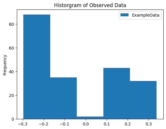
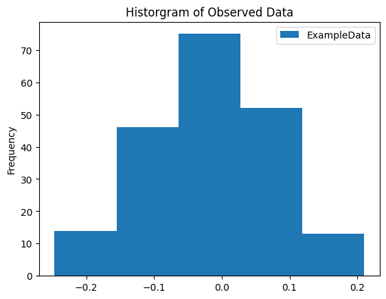
Generate a Histogram of Our Data
We observe a clear separation between signals in this plot.
1_ = observations.plot.hist(bins=5)
2_ = plt.title('Historgram of Observed Data')
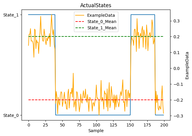
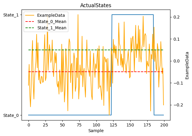
Plot States and Observations
Display our true states and the observed data we’ll be feeding to the model.
1_ = plot_states(actual_states, observations[NAME], obs_mean=EXAMPLE_MEAN, num_samples=NUM_SAMPLES)
Hidden Markov Model Setup
The hmm_cfg object is how we configure our Hidden Markov Model (HMM).
- We specify the number of expected states
- We specify what we are observing (there may be many, select the one we care about)
- We specify how to compute the expected emissions from each state
Computing the model state information is performed in a data-driven approach. We could randomly assign emission characteristics to each state, but that is less than ideal. We could assume some knowledge of how emissions and states relate and assign them manually, but that is cheating ;-P. So we let the data tell us what we should have; we want to understand what a typical emission from each state looks like and using a data-driven approach helps.
We use k-means clustering to initialize the emission parameters . K-means clusters our observations into N groups, providing initial estimates for the Mean and Variance of emissions generated by each state. This is just a starting point - Baum-Welch will refine these parameters during training. Note: this approach assumes that each state has a distinct emission profile (which is certainly not always the case in financial markets).
1hmm_cfg = HMMConfig(
2    n_states=N_STATES,
3    observed_signal=NAME,
4    initialization_method='kmeans'
5)
6hmm = HMM(hmm_cfg)
Fit the model
Once we have our data and model, we need to fit it to the data. The Baum-Welch algorithm is used to train the model by estimating the model parameters (transition probabilities and emission distribution parameters) that maximize the Likelihood
of observing our data. It does NOT determine state sequences - that’s what the Viterbi algorithm does (used later in .predict()). Baum-Welch uses the forward-backward algorithm
to iteratively refine the parameters until convergence. In our simple example with well-separated data, it should converge quickly (< 5 iterations).
1hmm.fit(observations)
Training on 200 observations (removed 0 NaN values)
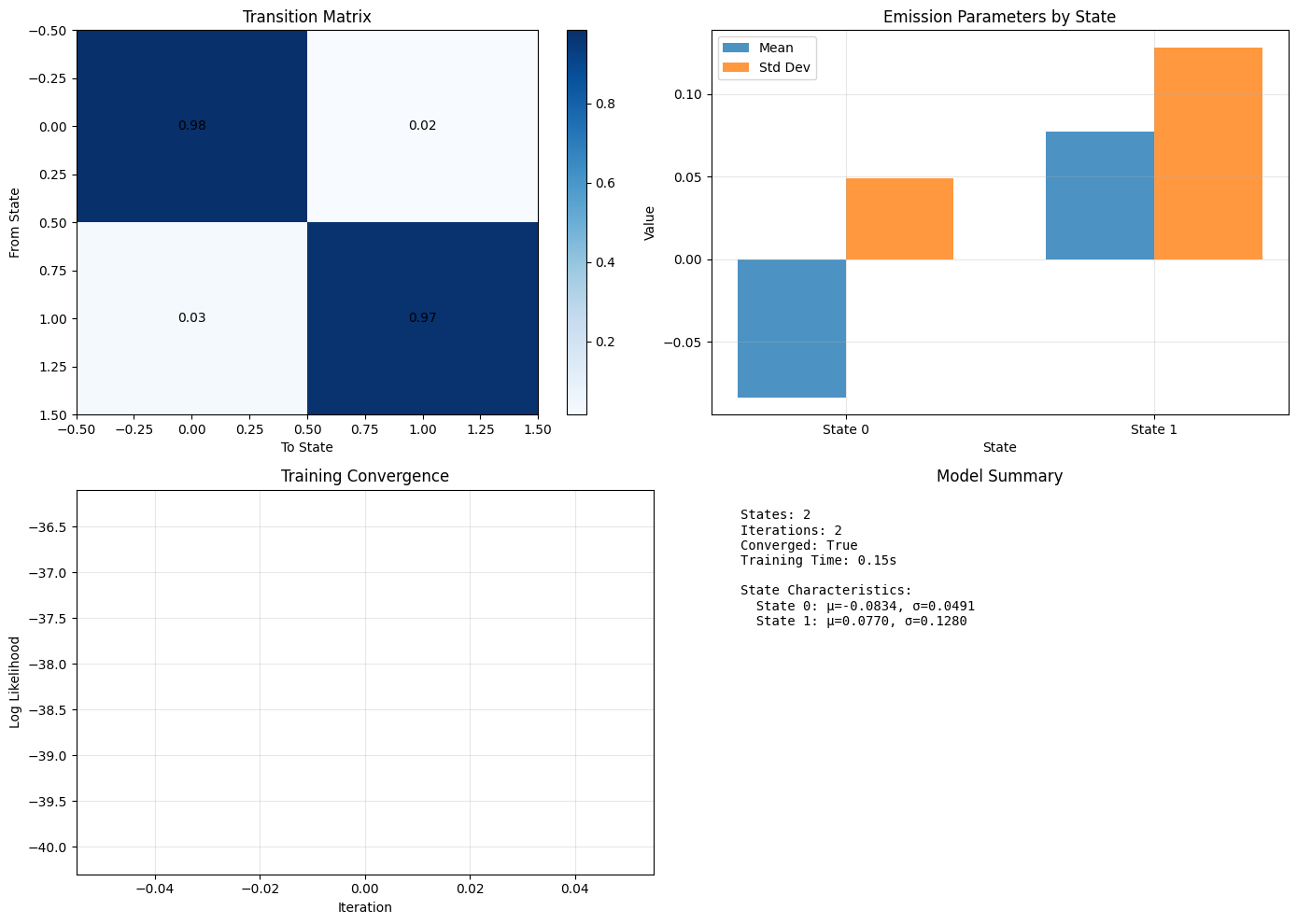
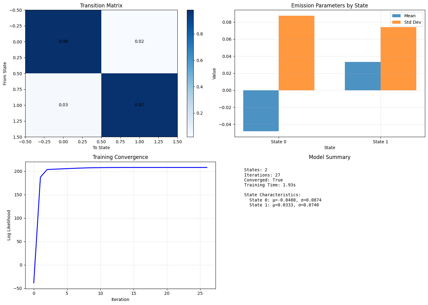
Visualize the Model
Now that we’ve fit the model, let’s understand what it thinks.
Transition Matrix tells us how likely state transitions are. Given how separated our data was, this should be very close to the identity matrix. When we repeat this with less separation in our data, this will become less distinct.
- When we have a matrix that is close to the identity, it indicates that the model will tend to remain in a state for a while (not very likely to change). Sidebar - if the transition matrix was truly identity, you would not have any state transitions.
- When we have a more uniformly distributed matrix, it indicates that the states will fluctuate at each time step.
Emission Parameters tells us what the model expects each state to produce.
Meanis the average value we expect from an observation in a given state. It should be close to theEXAMPLE_MEANvalue above.Std Devis the expected spread of an emission from a state (i.e., how a value varies from its mean). It should be close to theEXAMPLE_STDvalue above.
As we noted above, the Training Convergence plot is empty - this is expected given that we converged to a solution so quickly.
1_ = hmm.plot()
Make Predictions!
Ok, so we fit the model to the data. Let’s understand what it thought was happening and compare it to what we know actually happened.
1y = hmm.predict(observations)
Note: The
.predict()method uses the Viterbi algorithm to find the most likely state sequence given the trained model parameters. This is different from training - Viterbi decodes states, while Baum-Welch estimates parameters.
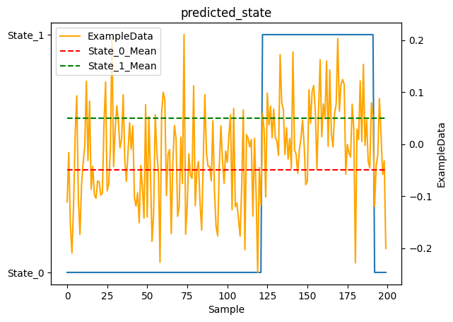
Prediction
As you can see, the model did pretty well! You would hope so, this is a very simple case. Let’s try again with something a bit more interesting.
1_ = plot_states(y.predicted_state, observations[NAME], obs_mean=EXAMPLE_MEAN, num_samples=NUM_SAMPLES)
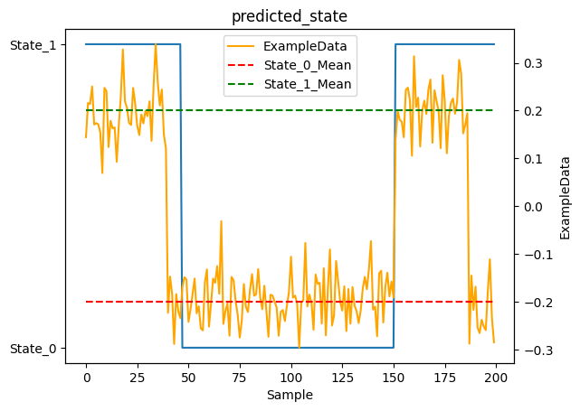
You’ll notice the model has some lag when transitioning from State_1 to State_0. This is expected behavior, not a bug! Here’s why:
The transition matrix is close to identity (diagonal values near 1), meaning states tend to persist. When the Viterbi algorithm decodes the state sequence, it performs a Bayesian calculation at each timestep, balancing:
- Emission evidence: “Does this observation look like it came from State X?”
- Transition prior: “How likely am I to be in State X given where I was before?”
When a true state change occurs, the first few observations after the change are ambiguous - they could plausibly come from either state. The algorithm needs to accumulate several observations that consistently favor the new state before the cumulative evidence overcomes the strong prior belief (encoded in the transition matrix) that states persist.
This is actually a feature! The lag prevents declaring state changes based on single noisy observations. In financial markets, this is desirable - you don’t want to declare a Regime change based on one unusual day. The lag provides natural smoothing and robustness to outliers.
1score = accuracy_score(actual_states, y.predicted_state)
2print(f"Accuracy score: {score:.3%}")
Accuracy score: 90.000%
1report = classification_report(actual_states, y.predicted_state)
2print("Classification Report:\n", report)
Classification Report:
               precision    recall  f1-score   support

           0       1.00      0.84      0.91       124
           1       0.79      1.00      0.88        76

    accuracy                           0.90       200
   macro avg       0.90      0.92      0.90       200
weighted avg       0.92      0.90      0.90       200
A More Complicated Problem
Let’s make the states less distinct and see how the model performs
1NEXT_EXAMPLE_MEAN = 0.05 # Closer centers for our emissions
2NEXT_EXAMPLE_STD = 0.08 # Fatter distribution of our emissions
1next_actual_states, next_observations = generate_observations(
2    obs_mean=NEXT_EXAMPLE_MEAN,
3    obs_std=NEXT_EXAMPLE_STD,
4    obs_name=NAME,
5    num_samples=NUM_SAMPLES)
Updated Observations
There is much less separation between the emissions generated by each of the states in our mixture now. This will be much more challenging for our model.
1_ = next_observations.plot.hist(bins=5)
2_ = plt.title('Historgram of Observed Data')
Observations
You can see the observations are much less distinct in this picture. There is some slight separation but given the increased variance in the signals it is tough to differentiate visually between the two states.
1_ = plot_states(next_actual_states, next_observations[NAME], obs_mean=NEXT_EXAMPLE_MEAN, num_samples=NUM_SAMPLES)
Model Update
Re-train our model on our latest observation set.
1hmm.fit(next_observations)
Training on 200 observations (removed 0 NaN values)
Training Results
You can see in the Training Convergence plot that it took much more effort for the model to become confident in its understanding of the data than the previous example. However, it was able to make reasonable assumptions about states and emission data despite the more “noisy” data.
1_ = hmm.plot()
Predictions!
Let’s see how we did given the more much more interesting problem…
1y = hmm.predict(next_observations)
1_ = plot_states(y.predicted_state, next_observations[NAME], obs_mean=NEXT_EXAMPLE_MEAN, num_samples=NUM_SAMPLES)
Analysis
The model was better than a coin-flip. Given the data in this example, that is a pretty good outcome! The observations were generated by the underlying states via their emission distributions, which were not very distinct; you’d be challenged to visually separate the mixture or identify which state produced which observation in this data set.
1score = accuracy_score(actual_states, y.predicted_state)
2print(f"Accuracy score: {score:.3%}")
Accuracy score: 63.000%
1report = classification_report(actual_states, y.predicted_state)
2print("Classification Report:\n", report)
Classification Report:
               precision    recall  f1-score   support

           0       0.69      0.73      0.71       124
           1       0.51      0.47      0.49        76

    accuracy                           0.63       200
   macro avg       0.60      0.60      0.60       200
weighted avg       0.62      0.63      0.63       200
Next Steps
So then, what can we do to improve our model in the face of difficult data?
| Step | Notes | Caution |
|---|---|---|
| More states | Adding more states to our model can help. | This comes at a price - model outputs are more difficult to interpret, model is more difficult to train. Also correlating emission characteristics to a state will be more challenging. |
| More data | Using more observations can help. | This is not always an option; we can’t just get more data from a stock for example. |
We’ll work through these in future posts.
Thanks for reading!