Hidden Regime Pipeline
Hidden Regime Pipeline
From Manual HMM to Production-Ready Pipeline
See the Notebook source on GitHub.
Your Learning Journey So Far
Notebook 1: Why Use Log Returns?
You learned WHY we use log returns:
- ✓ Stationarity (required for HMMs)
- ✓ Time additivity (returns simply add)
- ✓ Scale invariance (compare $60 and $500 stocks)
- ✓ Symmetric treatment (gains/losses balanced)
- ✓ Cross-asset comparability
Key Takeaway: Log returns aren’t convention—they’re mathematical necessity.
Notebook 2: HMM Basics
You learned HOW HMMs work:
- ✓ Hidden states represent market regimes
- ✓ Transition matrices capture regime persistence
- ✓ Emission parameters (μ, σ) define regime characteristics
- ✓ Viterbi algorithm finds most likely state sequence
- ✓ Forward-backward gives probability distributions
Key Takeaway: Don’t force “Bear/Bull” labels—let data reveal regimes.
Notebook 3: Production Pipeline (This Notebook)
You’ll learn USING the pipeline for real analysis:
- ✓ One-line pipeline setup (production efficiency)
- ✓ Automated regime labeling (threshold-based logic)
- ✓ Regime characteristics and persistence
- ✓ Choosing optimal number of states
- ✓ Best practices for regime detection
Scope Note: This notebook focuses on regime detection. For trading applications (risk management, position sizing, backtesting), see Notebook 4.
What This Notebook Covers
Part 1: Quick Pipeline Setup (Sections 1-2)
Part 2: Understanding Regime Classification (Sections 3-4)
Part 3: Regime Duration & Persistence (Section 5)
Part 4: Visualization (Section 6)
Part 5: Model Selection (Section 7)
Part 6: Best Practices & Next Steps (Section 8)
 1import sys
 2from pathlib import Path
 3import numpy as np
 4import pandas as pd
 5import matplotlib.pyplot as plt
 6import seaborn as sns
 7from datetime import datetime, timedelta
 8import warnings
 9warnings.filterwarnings('ignore')
10
11# Add parent to path
12sys.path.insert(0, str(Path().absolute().parent))
13
14# Import hidden_regime using the full API
15import hidden_regime as hr
16
17# Plotting
18plt.style.use('seaborn-v0_8-whitegrid')
19sns.set_palette(sns.color_palette())
20
21print("Imports complete")
22print(f"hidden-regime version: {hr.__version__}")
Imports complete
hidden-regime version: 1.0.0
1. Quick Start: Pipeline Factory
The library provides factory functions for quick pipeline creation.
 1# Create a complete financial pipeline with one function call
 2ticker = 'NVDA'
 3n_states = 3
 4
 5pipeline = hr.create_financial_pipeline(
 6    ticker=ticker,
 7    n_states=n_states,
 8    include_report=False  # We'll do custom analysis
 9)
10
11# Display pipeline components
12print(f"Pipeline created for {ticker} with {n_states} states")
13print(f"  Data loader: {type(pipeline.data).__name__}")
14print(f"  Observations: {type(pipeline.observation).__name__}")
15print(f"  Model: {type(pipeline.model).__name__}")
16print(f"  Analysis: {type(pipeline.analysis).__name__}")
Pipeline created for NVDA with 3 states
  Data loader: FinancialDataLoader
  Observations: FinancialObservationGenerator
  Model: HiddenMarkovModel
  Analysis: FinancialAnalysis
2. Run the Complete Pipeline
The pipeline.update() method executes all stages:
- Data loading: Downloads historical price data
- Observation generation: Computes log returns
- Model training: Fits HMM using Baum-Welch algorithm
- Analysis: Generates regime classifications and metrics
1# Execute pipeline
2report = pipeline.update()
3
4# Get analysis results
5result = pipeline.component_outputs['analysis']
6
7# Display summary
8print(f"Analysis complete: {result.shape[0]} days, {result.shape[1]} metrics")
9print(f"Date range: {result.index[0].date()} to {result.index[-1].date()}")
Training on 500 observations (removed 0 NaN values)
Analysis complete: 500 days, 37 metrics
Date range: 2023-10-17 to 2025-10-14
3. Threshold-Based Regime Mapping
How Regimes Are Classified
The library uses data-driven thresholds on emission means $\mu_k$:
$ \text{regime}_k = \begin{cases} \text{Bear} & \text{if } \mu_k < \theta_{\text{bear}} \\ \text{Bull} & \text{if } \mu_k > \theta_{\text{bull}} \\ \text{Sideways} & \text{otherwise} \end{cases} $
Where $\theta_{\text{bear}}$ and $\theta_{\text{bull}}$ are determined by:
- Historical return distributions
- Volatility-adjusted cutoffs
- Statistical significance tests
Key Point: We do NOT sort states by index and assign “State 0 = Bear, State 1 = Sideways, State 2 = Bull”. The data reveals the regime types.
  1# Get raw data with log returns
  2raw_data = pipeline.data.get_all_data()
  3
  4# Find log_return column (case-insensitive)
  5log_return_col = None
  6for col in raw_data.columns:
  7    if col.lower() == 'log_return':
  8        log_return_col = col
  9        break
 10
 11# Prepare regime data for visualization
 12regimes = result['regime_name'].unique()
 13regime_stats = []
 14
 15for regime in sorted(regimes):
 16    regime_data = result[result['regime_name'] == regime]
 17    n_days = len(regime_data)
 18    pct_time = n_days / len(result) * 100
 19    state_num = regime_data['predicted_state'].iloc[0]
 20
 21    stats = {
 22        'regime': regime,
 23        'state': state_num,
 24        'days': n_days,
 25        'pct_time': pct_time
 26    }
 27
 28    # Get log returns for this regime by aligning indices
 29    if log_return_col is not None:
 30        regime_indices = regime_data.index
 31        obs_returns = raw_data.loc[regime_indices, log_return_col].dropna()
 32
 33        if len(obs_returns) > 0:
 34            avg_log = obs_returns.mean()
 35            avg_pct = hr.log_return_to_percent_change(avg_log) * 100
 36            vol_daily = obs_returns.std() * 100
 37            vol_annual = vol_daily * np.sqrt(252)
 38
 39            stats.update({
 40                'daily_return': avg_pct,
 41                'daily_vol': vol_daily,
 42                'annual_return': avg_pct * 252,
 43                'annual_vol': vol_annual
 44            })
 45
 46    regime_stats.append(stats)
 47
 48# Create visualization with larger figure size
 49fig, (ax1, ax2) = plt.subplots(1, 2, figsize=(18, 7))
 50
 51# Get regime colors
 52unique_regimes = sorted(result['regime_name'].unique())
 53from hidden_regime.visualization import get_regime_colors
 54color_list = get_regime_colors(len(unique_regimes), color_scheme="colorblind_safe")
 55regime_colors = dict(zip(unique_regimes, color_list))
 56
 57# Left: Pie chart of regime distribution
 58sizes = [s['pct_time'] for s in regime_stats]
 59labels = [f"{s['regime']}\n{s['pct_time']:.1f}%" for s in regime_stats]
 60colors = [regime_colors[s['regime']] for s in regime_stats]
 61
 62wedges, texts, autotexts = ax1.pie(sizes, labels=labels, colors=colors, autopct='',
 63                                     startangle=90, textprops={'fontsize': 13, 'fontweight': 'bold'})
 64ax1.set_title('Regime Distribution\n(% of Time)', fontsize=15, fontweight='bold', pad=20)
 65
 66# Right: Bar chart of returns by regime
 67regime_names = [s['regime'] for s in regime_stats]
 68returns = [s.get('annual_return', 0) for s in regime_stats]
 69bar_colors = [regime_colors[s['regime']] for s in regime_stats]
 70
 71bars = ax2.barh(regime_names, returns, color=bar_colors, alpha=0.7, edgecolor='black', linewidth=1.5)
 72ax2.axvline(x=0, color='black', linestyle='-', linewidth=0.8)
 73ax2.set_xlabel('Annualized Return (%)', fontsize=13)
 74ax2.set_ylabel('Regime', fontsize=13)
 75ax2.set_title('Expected Returns by Regime', fontsize=15, fontweight='bold', pad=20)
 76ax2.grid(True, alpha=0.3, axis='x')
 77ax2.tick_params(axis='both', labelsize=12)
 78
 79# Add value labels on bars
 80for i, (bar, val) in enumerate(zip(bars, returns)):
 81    if val != 0:  # Only add label if we have data
 82        label_x = val + (3 if val > 0 else -3)
 83        ha = 'left' if val > 0 else 'right'
 84        ax2.text(label_x, bar.get_y() + bar.get_height()/2,
 85                 f'{val:+.1f}%', ha=ha, va='center', fontweight='bold', fontsize=12)
 86
 87plt.tight_layout()
 88plt.show()
 89
 90# Print detailed statistics
 91print("\nDetailed Regime Characteristics")
 92print("=" * 80)
 93for s in regime_stats:
 94    print(f"\n{s['regime']} (State {s['state']})")
 95    print("-" * 80)
 96    print(f"  Frequency:   {s['days']} days ({s['pct_time']:.1f}% of period)")
 97    if 'daily_return' in s:
 98        print(f"  Daily:       mu = {s['daily_return']:+.3f}%  sigma = {s['daily_vol']:.3f}%")
 99        print(f"  Annualized:  mu = {s['annual_return']:+.1f}%  sigma = {s['annual_vol']:.1f}%")
100print("=" * 80)
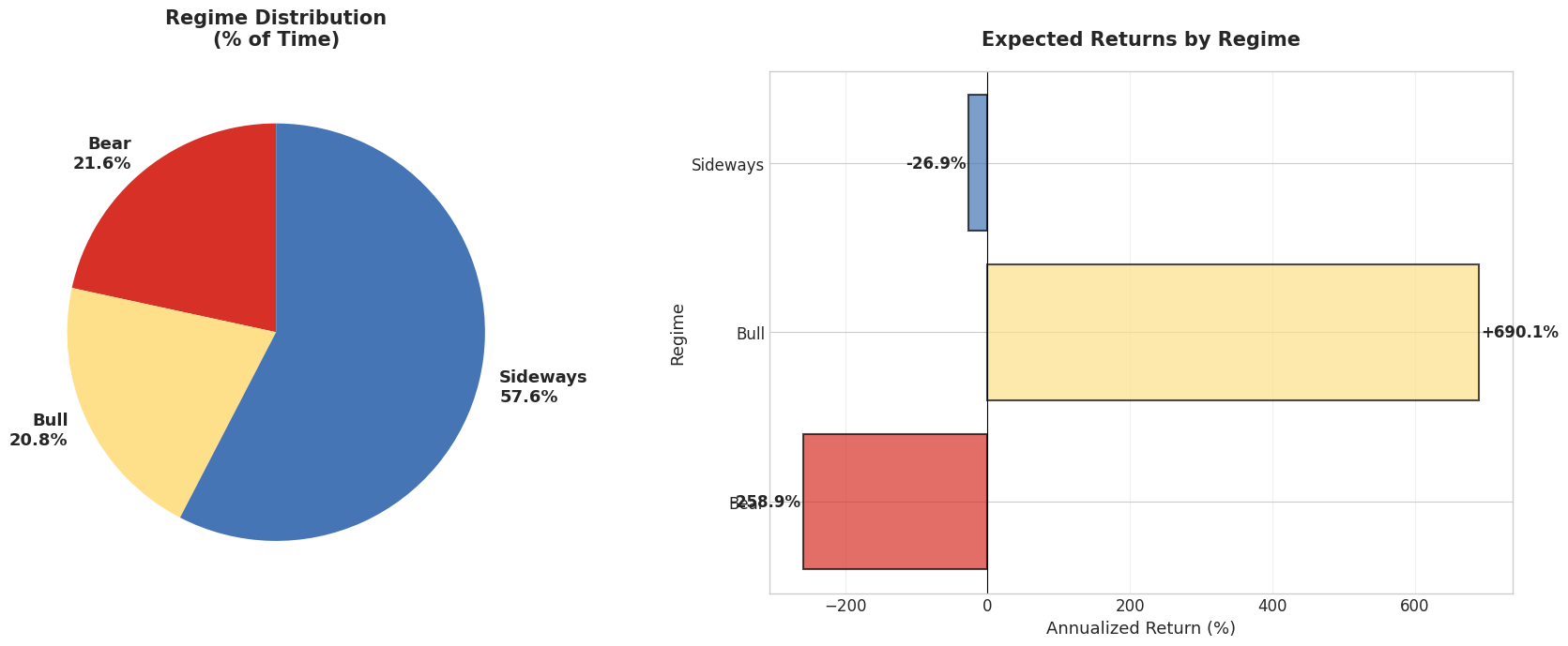
Detailed Regime Characteristics
================================================================================

Bear (State 0)
--------------------------------------------------------------------------------
  Frequency:   108 days (21.6% of period)
  Daily:       mu = -1.027%  sigma = 4.131%
  Annualized:  mu = -258.9%  sigma = 65.6%

Bull (State 2)
--------------------------------------------------------------------------------
  Frequency:   104 days (20.8% of period)
  Daily:       mu = +2.739%  sigma = 1.221%
  Annualized:  mu = +690.1%  sigma = 19.4%

Sideways (State 1)
--------------------------------------------------------------------------------
  Frequency:   288 days (57.6% of period)
  Daily:       mu = -0.107%  sigma = 1.356%
  Annualized:  mu = -26.9%  sigma = 21.5%
================================================================================
4. Current Regime Status
State Probability Distribution
The HMM provides full probability distribution at each time point:
$ P(\text{state}_k \mid O_1, \ldots, O_T) = \frac{\alpha_T(k) \beta_T(k)}{\sum_{j} \alpha_T(j) \beta_T(j)} $
Where:
- $\alpha_t(k)$: Forward probability (probability of observations up to $t$ AND being in state $k$)
- $\beta_t(k)$: Backward probability (probability of future observations GIVEN state $k$ at $t$)
Confidence is the maximum probability: $\max_k P(\text{state}_k \mid \text{all data})$
 1# Analyze current regime
 2current = result.iloc[-1]
 3current_regime = current['regime_name']
 4
 5# Count consecutive days in regime
 6days_in_regime = 1
 7for i in range(len(result)-2, -1, -1):
 8    if result.iloc[i]['regime_name'] == current_regime:
 9        days_in_regime += 1
10    else:
11        break
12
13# Get state probabilities
14state_probs = []
15state_names = []
16for state in range(n_states):
17    col_name = f'state_{state}_prob'
18    if col_name in result.columns:
19        prob = current[col_name]
20        # Find regime name for this state
21        state_regime = result[result['predicted_state'] == state]['regime_name'].iloc[0] \
22                      if len(result[result['predicted_state'] == state]) > 0 else f"State {state}"
23        state_probs.append(prob)
24        state_names.append(state_regime)
25
26# Create bar chart
27fig, ax = plt.subplots(figsize=(12, 5))
28
29# Get colors for bars
30unique_regimes = sorted(result['regime_name'].unique())
31from hidden_regime.visualization import get_regime_colors
32color_list = get_regime_colors(len(unique_regimes), color_scheme="colorblind_safe")
33regime_colors = dict(zip(unique_regimes, color_list))
34bar_colors = [regime_colors.get(name, 'gray') for name in state_names]
35
36# Create horizontal bar chart
37bars = ax.barh(state_names, state_probs, color=bar_colors, alpha=0.7, edgecolor='black', linewidth=2)
38
39# Highlight the current regime (max probability)
40max_idx = np.argmax(state_probs)
41bars[max_idx].set_alpha(1.0)
42bars[max_idx].set_linewidth(3)
43
44# Add percentage labels
45for i, (bar, prob) in enumerate(zip(bars, state_probs)):
46    ax.text(prob + 0.02, bar.get_y() + bar.get_height()/2,
47            f'{prob*100:.1f}%', ha='left', va='center', fontweight='bold', fontsize=11)
48
49# Formatting
50ax.set_xlim(0, 1.1)
51ax.set_xlabel('Probability', fontsize=12)
52ax.set_title(f'Current Market Regime: {current_regime} ' +
53             f'(Confidence: {current["confidence"]*100:.1f}%)',
54             fontsize=14, fontweight='bold', pad=15)
55ax.grid(True, alpha=0.3, axis='x')
56
57# Add vertical line at confidence threshold
58ax.axvline(x=0.8, color='green', linestyle='--', alpha=0.5, linewidth=2, label='High confidence (>80%)')
59ax.legend(loc='lower right')
60
61plt.tight_layout()
62plt.show()
63
64# Print summary
65print(f"\nCurrent Market Status")
66print("=" * 70)
67print(f"  Date:       {result.index[-1].date()}")
68print(f"  Regime:     {current_regime}")
69print(f"  Confidence: {current['confidence']*100:.1f}%")
70print(f"  Duration:   {days_in_regime} days in current regime")
71print("=" * 70)
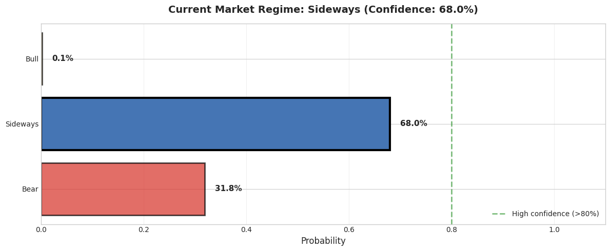
Current Market Status
======================================================================
  Date:       2025-10-14
  Regime:     Sideways
  Confidence: 68.0%
  Duration:   24 days in current regime
======================================================================
5. Regime Duration Analysis
Expected Regime Duration
From the HMM transition matrix $\mathbf{A}$, the expected duration in regime $k$ is:
$ E[\tau_k] = \frac{1}{1 - A_{kk}} $
Where $A_{kk} = P(\text{state}_{t+1} = k \mid \text{state}_t = k)$ is the probability of staying in the same regime.
Example: If $A_{kk} = 0.90$, then $E[\tau] = \frac{1}{1-0.90} = 10$ days.
Why Duration Matters
- Short regimes (1-3 days): Possible overfitting or high-frequency market noise
- Medium regimes (5-15 days): Typical market regime persistence
- Long regimes (20+ days): Strong, stable market conditions
Duration analysis validates that the HMM is finding real market patterns, not random noise.
 1# Calculate regime durations
 2def calculate_regime_durations(df):
 3    """Calculate duration of each regime period"""
 4    durations = []
 5    current_regime = df.iloc[0]['regime_name']
 6    current_duration = 1
 7
 8    for i in range(1, len(df)):
 9        if df.iloc[i]['regime_name'] == current_regime:
10            current_duration += 1
11        else:
12            durations.append({
13                'regime': current_regime,
14                'duration': current_duration,
15                'start': df.index[i-current_duration],
16                'end': df.index[i-1]
17            })
18            current_regime = df.iloc[i]['regime_name']
19            current_duration = 1
20
21    # Add final period
22    durations.append({
23        'regime': current_regime,
24        'duration': current_duration,
25        'start': df.index[len(df)-current_duration],
26        'end': df.index[-1]
27    })
28
29    return pd.DataFrame(durations)
30
31durations_df = calculate_regime_durations(result)
32
33# Display statistics
34print("Regime Duration Statistics")
35print("=" * 70)
36print(f"Total regime transitions: {len(durations_df)}\n")
37
38for regime in sorted(durations_df['regime'].unique()):
39    regime_durs = durations_df[durations_df['regime'] == regime]['duration']
40
41    print(f"{regime}:")
42    print(f"  Occurrences: {len(regime_durs)} periods")
43    print(f"  Average:     {regime_durs.mean():.1f} days  (median: {regime_durs.median():.0f})")
44    print(f"  Range:       {regime_durs.min()} - {regime_durs.max()} days")
45    print()
46
47# Show longest periods
48print("Longest Regime Periods:")
49print("-" * 70)
50longest = durations_df.nlargest(5, 'duration')
51for idx, row in longest.iterrows():
52    print(f"  {row['regime']:<12} {row['duration']:>3} days  " +
53          f"({row['start'].date()} → {row['end'].date()})")
54print("=" * 70)
Regime Duration Statistics
======================================================================
Total regime transitions: 75

Bear:
  Occurrences: 11 periods
  Average:     9.8 days  (median: 6)
  Range:       1 - 40 days

Bull:
  Occurrences: 32 periods
  Average:     3.2 days  (median: 3)
  Range:       1 - 10 days

Sideways:
  Occurrences: 32 periods
  Average:     9.0 days  (median: 5)
  Range:       1 - 39 days

Longest Regime Periods:
----------------------------------------------------------------------
  Bear          40 days  (2025-02-24 → 2025-04-21)
  Sideways      39 days  (2025-07-16 → 2025-09-09)
  Sideways      34 days  (2023-11-15 → 2024-01-04)
  Sideways      24 days  (2025-09-11 → 2025-10-14)
  Sideways      22 days  (2024-11-20 → 2024-12-20)
======================================================================
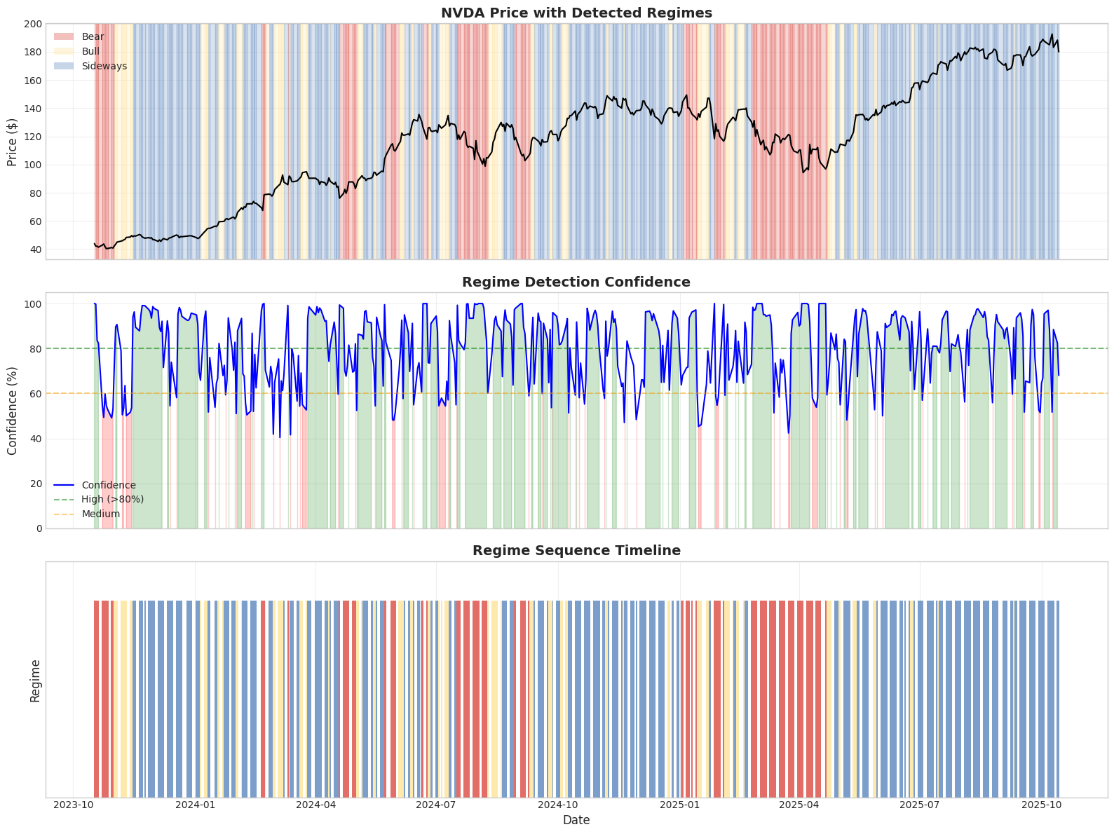
6. Visualization
Three-panel visualization showing:
- Price with regime shading: Visual alignment of regimes with price action
- Confidence levels: How certain the model is about each regime
- Regime timeline: Sequential regime transitions
 1# Create regime visualization
 2fig, axes = plt.subplots(3, 1, figsize=(16, 12), sharex=True)
 3
 4# Get raw price data
 5raw_data = pipeline.data.get_all_data()
 6close_col = next((col for col in raw_data.columns if col.lower() == 'close'), None)
 7
 8if close_col is None:
 9    raise ValueError("Could not find 'close' column in data")
10
11# Get regime colors
12unique_regimes = sorted(result['regime_name'].unique())
13from hidden_regime.visualization import get_regime_colors
14color_list = get_regime_colors(len(unique_regimes), color_scheme="colorblind_safe")
15regime_colors = dict(zip(unique_regimes, color_list))
16
17# Panel 1: Price with regime shading
18ax = axes[0]
19ax.plot(raw_data.index, raw_data[close_col], linewidth=1.5, color='black', zorder=2)
20ax.set_ylabel('Price ($)', fontsize=12)
21ax.set_title(f'{ticker} Price with Detected Regimes', fontsize=14, fontweight='bold')
22ax.grid(True, alpha=0.3)
23
24# Shade background by regime
25for i in range(len(result)):
26    regime = result.iloc[i]['regime_name']
27    color = regime_colors.get(regime, 'gray')
28    ax.axvspan(result.index[i], result.index[min(i+1, len(result)-1)],
29               alpha=0.2, color=color, zorder=1)
30
31# Add legend
32from matplotlib.patches import Patch
33legend_elements = [Patch(facecolor=regime_colors.get(r, 'gray'), alpha=0.3, label=r)
34                   for r in unique_regimes]
35ax.legend(handles=legend_elements, loc='upper left')
36
37# Panel 2: Confidence levels
38ax = axes[1]
39confidence_pct = result['confidence'] * 100
40
41ax.plot(result.index, confidence_pct, linewidth=1.5, color='blue', label='Confidence')
42ax.axhline(y=80, color='green', linestyle='--', alpha=0.5, label='High (>80%)')
43ax.axhline(y=60, color='orange', linestyle='--', alpha=0.5, label='Medium')
44
45# Shade confidence regions
46ax.fill_between(result.index, 0, confidence_pct,
47                where=(confidence_pct > 80), alpha=0.2, color='green')
48ax.fill_between(result.index, 0, confidence_pct,
49                where=(confidence_pct < 60), alpha=0.2, color='red')
50
51ax.set_ylabel('Confidence (%)', fontsize=12)
52ax.set_title('Regime Detection Confidence', fontsize=14, fontweight='bold')
53ax.grid(True, alpha=0.3)
54ax.legend(loc='lower left')
55ax.set_ylim(0, 105)
56
57# Panel 3: Regime timeline
58ax = axes[2]
59for i in range(len(result)):
60    regime = result.iloc[i]['regime_name']
61    color = regime_colors.get(regime, 'gray')
62    ax.bar(result.index[i], 1, width=1, color=color, edgecolor='none', alpha=0.7)
63
64ax.set_ylabel('Regime', fontsize=12)
65ax.set_xlabel('Date', fontsize=12)
66ax.set_title('Regime Sequence Timeline', fontsize=14, fontweight='bold')
67ax.set_ylim(0, 1.2)
68ax.set_yticks([])
69ax.grid(True, alpha=0.3, axis='x')
70
71plt.tight_layout()
72plt.show()
7. Model Comparison
Selecting Optimal Number of States
Model complexity tradeoff:
- Too few states: Cannot capture market nuances
- Too many states: Overfitting, very short regimes
Validation metrics:
- Average duration: Should be 5+ days for meaningful regimes
- Confidence: Higher confidence indicates clearer regime separation
- Number of parameters: $n_{\text{params}} = n^2 + 2n$ for $n$ states
- Interpretability: Can you explain what each regime represents?
 1# Compare models with different numbers of states
 2comparison_results = []
 3
 4print("Training models with 2-5 states...\n")
 5
 6for n in [2, 3, 4, 5]:
 7    print(f"  {n} states... ", end='', flush=True)
 8
 9    test_pipeline = hr.create_financial_pipeline(
10        ticker=ticker,
11        n_states=n,
12        include_report=False
13    )
14
15    _ = test_pipeline.update()
16    test_result = test_pipeline.component_outputs['analysis']
17
18    # Calculate metrics
19    n_params = n**2 + 2*n  # Transitions + emissions
20    n_obs = len(test_result)
21    switches = (test_result['predicted_state'].diff() != 0).sum()
22    avg_duration = n_obs / switches if switches > 0 else n_obs
23    avg_conf = test_result['confidence'].mean() * 100
24
25    comparison_results.append({
26        'States': n,
27        'Parameters': n_params,
28        'Switches': switches,
29        'Avg Duration': f"{avg_duration:.1f}",
30        'Avg Confidence': f"{avg_conf:.1f}%"
31    })
32
33    print("done")
34
35# Display comparison table
36comp_df = pd.DataFrame(comparison_results)
37print("\n" + "=" * 70)
38print("Model Comparison Results")
39print("=" * 70)
40print(comp_df.to_string(index=False))
41print("=" * 70)
Training models with 2-5 states...

  2 states... Training on 500 observations (removed 0 NaN values)
done
  3 states... Training on 500 observations (removed 0 NaN values)
done
  4 states... Training on 500 observations (removed 0 NaN values)
done
  5 states... Training on 500 observations (removed 0 NaN values)
done

======================================================================
Model Comparison Results
======================================================================
 States  Parameters  Switches Avg Duration Avg Confidence
      2           8        24         20.8          89.2%
      3          15        75          6.7          79.5%
      4          24       101          5.0          78.8%
      5          35       114          4.4          78.7%
======================================================================
Selection Guidelines
Interpreting the results:
| States | Typical Use Case | Watch Out For |
|---|---|---|
| 2 | Simple bull/bear classification | May miss sideways markets |
| 3 | Bear/Sideways/Bull (recommended) | Good balance |
| 4 | Adding crisis or rally states | Check duration > 5 days |
| 5+ | Very granular regimes | Often overfits, short regimes |
Red flags:
- ⚠️ Average duration < 5 days → Likely overfitting
- ⚠️ Confidence < 60% → Poor regime separation
- ⚠️ Too many switches → Capturing noise, not signal
Recommended: Start with 3 states. Add more only if:
- Durations remain meaningful (>5 days)
- Each regime has clear interpretation
- Validation on out-of-sample data shows improvement
7. Model Comparison
Compare different numbers of states to find the optimal model complexity.
8. Best Practices for Regime Detection
✓ DO These Things
1. Always Use Log Returns
- Ensures stationarity (required for HMMs)
- Proper statistical properties
- Cross-asset comparability
2. Let Data Determine Regimes
- Use threshold-based classification
- Don’t force “Bear/Bull” labels by sorting state indices
- Examine emission parameters before labeling
3. Check Confidence Levels
- Low confidence → regime uncertainty or transitions
- High confidence → reliable regime signals
- Use confidence for position sizing
4. Validate Regime Duration
- Very short regimes (< 3 days) → possible overfitting
- Typical regimes (5-15 days) → reasonable persistence
- Long regimes (20+ days) → strong, stable conditions
5. Compare Multiple Models
- Try 2-5 states systematically
- Balance fit quality vs complexity
- Use validation metrics (duration, confidence)
6. Monitor Regime Changes
- Large parameter shifts → market structure changes
- Regime transition patterns → leading indicators
- Confidence drops → early warning signals
⚠️ DON’T Do These Things
1. Don’t Use Raw Prices
- Prices are non-stationary
- Violates HMM assumptions
- Produces invalid inferences
2. Don’t Force Regime Labels
- State 0 ≠ automatically “Bear”
- Let emission means determine regime types
- Thresholds should be data-driven
3. Don’t Ignore Low Confidence
- Low confidence carries information
- Often signals regime transitions
- Critical for risk management
4. Don’t Assume Stationarity
- Market regimes evolve over time
- Parameters change with market structure
- Regular retraining may be needed
5. Don’t Overtrain
- More states ≠ better model
- 5+ states often overfit
- Focus on interpretability
6. Don’t Use Single Random Seed
- HMMs have local optima
- Results can vary by initialization
- Consider multiple runs or robust initialization
Production Checklist
Before deploying for real trading decisions:
- Verified log returns are used (not prices or simple returns)
- Checked regime durations are reasonable (not too short)
- Validated confidence levels are meaningful
- Compared 2-5 states and selected optimal complexity
- Examined regime characteristics match market intuition
- Tested on out-of-sample data
- Established monitoring for regime changes
- Integrated with risk management system (see Notebook 4)
9. Conclusion & Next Steps
What You’ve Accomplished
Congratulations! You now have a complete understanding of regime detection using HMMs:
From Notebook 1 (Mathematical Foundation):
- ✓ Why log returns are mathematically necessary
- ✓ Stationarity, additivity, and scale invariance
- ✓ Properties required for statistical modeling
From Notebook 2 (HMM Mechanics):
- ✓ How HMMs represent market regimes
- ✓ What transition matrices and emissions mean
- ✓ Viterbi vs forward-backward algorithms
- ✓ Interpreting states without forcing labels
From Notebook 3 (Production Pipeline) - This Notebook:
- ✓ One-line pipeline setup
- ✓ Automated threshold-based regime classification
- ✓ Regime duration and persistence analysis
- ✓ Model selection (2-5 states comparison)
- ✓ Visualization and interpretation
- ✓ Best practices for production use
The Complete Learning Path
Notebook 1: Mathematical Foundation (WHY)
    ↓
Notebook 2: HMM Mechanics (HOW)
    ↓
Notebook 3: Production Pipeline (USING) ← You are here
    ↓
Notebook 4: Trading Applications (PROFITING) ← Next step
What’s Next: Notebook 4 - Advanced Trading Applications
You can now detect regimes. Notebook 4 teaches you how to USE them for trading:
Part A: Regime-Specific Risk Management
- VaR and Expected Shortfall by regime
- Maximum drawdown analysis
- Sharpe ratios and risk-adjusted returns
- Dynamic position sizing based on regime risk
Part B: Technical Indicator Integration
- Combining HMM regimes with RSI, MACD, Bollinger Bands
- Agreement/disagreement analysis
- When to trust HMMs vs indicators
- Ensemble signal generation
Part C: Portfolio Applications
- Position signals (LONG/SHORT/NEUTRAL)
- Confidence-weighted position sizing
- Signal strength methodology
- Risk-adjusted portfolio allocation
Part D: Backtesting & Validation
- Hypothetical performance comparison
- Walk-forward analysis
- Regime-based strategy testing
- Out-of-sample validation
Practical Next Steps
If you want to continue learning:
- Open Notebook 4 to learn trading applications
- Apply these techniques to your own tickers
- Experiment with different time periods
- Try different numbers of states
If you’re ready for production:
- Review the best practices checklist above
- Test on multiple assets and time periods
- Validate regime stability over time
- Integrate with your existing trading system
- Start with paper trading before real capital
If you want to customize:
- Modify threshold values for regime classification
- Add your own features beyond log returns
- Implement custom risk metrics
- Integrate with other analysis tools
Key Takeaways
Regime detection is a tool, not a crystal ball.
Use it to:
- Understand current market conditions
- Adjust risk based on regime characteristics
- Combine with other analysis methods
- Make more informed trading decisions
Don’t expect it to:
- Predict future price movements perfectly
- Work in all market conditions
- Replace fundamental analysis
- Guarantee profitable trades
Resources
- Documentation: Hidden Regime Docs
- Examples: More examples in
/examplesdirectory - Issues: Report bugs at GitHub
- Community: Share strategies and learn from others
Ready for trading applications? Open Notebook 4!